Please Note: This article is written for users of the following Microsoft Excel versions: 97, 2000, 2002, and 2003. If you are using a later version (Excel 2007 or later), this tip may not work for you. For a version of this tip written specifically for later versions of Excel, click here: Freezing Top Rows and Bottom Rows.
Kevin has a long (vertical) worksheet that has the first few rows frozen so the column headings are always visible. He would like to also freeze the bottom row, so the column totals are always visible.
Unfortunately there is no way to do this in Excel. At first thought you may believe that you can freeze rows and also split the worksheet window so that you can put the totals below the split. Excel won't let you do this, however—when you try, then the freeze is removed and replaced with the split, and trying to reapply the freeze removes the split.
What most experienced Excel users do is to put the column totals at the top of the columns instead of at the bottom. This may seem awkward, but it has the added benefit of allowing you to easily add new rows to your data table. The top-of-column totals could be added either using SUM formulas (as you would with the totals at the bottom), or you can leave the totals at the bottom of the columns and simply add a referential formula (like =B327) in a row at the top of columns.
There is another approach you can use, however. Start by opening the workbook that contains the worksheet you want to work on. (This should be the only workbook open.) Then follow these steps:
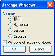
Figure 1. The Arrange Windows dialog box.
At this point you should see your two windows—one in the top half of the screen and the other beneath it. Use the mouse to adjust the vertical height of both windows. (The bottom window should be large enough to hold your totals and the top window can occupy the rest of the available space.)
Now you can display the totals row (or rows) in the bottom window, and freeze the top rows in the top window. This allows you to see everything you want to see, although it is a bit expensive when it comes to screen real estate since both windows have column letters visible.
The biggest drawback to this approach is that the windows are not horizontally linked. This means that if you scroll one of the windows left or right, the other window doesn't scroll at the same time. You could write some VBA code to handle the horizontal scrolling, but that simple adds complexity to the situation.
ExcelTips is your source for cost-effective Microsoft Excel training. This tip (3286) applies to Microsoft Excel 97, 2000, 2002, and 2003. You can find a version of this tip for the ribbon interface of Excel (Excel 2007 and later) here: Freezing Top Rows and Bottom Rows.

Best-Selling VBA Tutorial for Beginners Take your Excel knowledge to the next level. With a little background in VBA programming, you can go well beyond basic spreadsheets and functions. Use macros to reduce errors, save time, and integrate with other Microsoft applications. Fully updated for the latest version of Office 365. Check out Microsoft 365 Excel VBA Programming For Dummies today!
Need to move quickly through the worksheets in a workbook? Learn the keyboard shortcuts and you can make short work of ...
Discover MoreIf you need to save your Excel data at different benchmarks, you might want to use some sort of "versioning" system. Such ...
Discover MoreDo you need to pull a particular worksheet out of a group of workbooks and combine those worksheets into a different ...
Discover MoreFREE SERVICE: Get tips like this every week in ExcelTips, a free productivity newsletter. Enter your address and click "Subscribe."
There are currently no comments for this tip. (Be the first to leave your comment—just use the simple form above!)
Got a version of Excel that uses the menu interface (Excel 97, Excel 2000, Excel 2002, or Excel 2003)? This site is for you! If you use a later version of Excel, visit our ExcelTips site focusing on the ribbon interface.
FREE SERVICE: Get tips like this every week in ExcelTips, a free productivity newsletter. Enter your address and click "Subscribe."
Copyright © 2026 Sharon Parq Associates, Inc.
 Please Note:
This article is written for users of the following Microsoft Excel versions: 97, 2000, 2002, and 2003. If you are using a later version (Excel 2007 or later), this tip may not work for you. For a version of this tip written specifically for later versions of Excel, click here:
Please Note:
This article is written for users of the following Microsoft Excel versions: 97, 2000, 2002, and 2003. If you are using a later version (Excel 2007 or later), this tip may not work for you. For a version of this tip written specifically for later versions of Excel, click here:
Comments