Copying Formulas using a Pattern

Suppose you have a worksheet that contains a series of formulas in cells A1:A3. Cell A1 contains the formula =Sheet1!B4, cell A2 contains =Sheet1!B18, and cell A3 contains =Sheet1!B32. You might need to continue this pattern down the column, such that A4 contains =Sheet1!B46, etc.

The problem is, if you simply copy the cells, the pattern isn't continued. Instead, the formulas are adjusted based on the target cell's relation to the source cell. Thus, if you paste A1:A3 into A4:A6, then A4 will contain =Sheet1!B7, which is not what you want. (This happens whether you specifically copy and paste or fill the cells by dragging the fill handle.)

There is no way to continue a pattern while copying a formula. Instead, you need to revisit how you put the formula together in the first place. For instance, consider this formula:

=INDIRECT("Sheet1!B"&((ROW()-1)*14)+4)

This formula constructs a reference based on the position of the cell in which the formula is placed. If this formula is placed in cell A1, then the ROW function returns 1, the row in which the formula is placed. Thus, the formula becomes this:

=INDIRECT("Sheet1!B"&((1-1)*14)+4)
=INDIRECT("Sheet1!B"&(0*14)+4)
=INDIRECT("Sheet1!B"&0+4)
=INDIRECT("Sheet1!B"&4)
=INDIRECT("Sheet1!B4")

What is returned is the value at Sheet1!B4, just as originally wanted. When you copy this formula down the column, however, the ROW function returns something different in each row. In effect, the ROW function becomes a way to increase the offset of each formula by 14 rows from the one before it--just what you wanted.

You can also use a slightly different approach, this time using the OFFSET function:

=OFFSET(Sheet1!$B$4,(ROW()-1)*14,0)

This formula grabs a value based on the row in which the formula is placed (again, using the ROW function) and offset from cell Sheet1!B4. Placed into the first row of a column and then copied down that column, the formula returns values according to the pattern desired.

Another approach is to create the desired formulas directly. You can best do this by following these steps:

1. Start with a new, blank worksheet in a workbook containing a worksheet named "Sheet1."
2. In cell A1 enter the formula =Sheet1!B4.
3. Since the formula pattern is every 14 rows, highlight the range A1:A14. Only the first cell should have the formula; the other 13 are blank.
4. Drag the fill handle (the small square at the lower-right corner of the selection downward for a good number of rows--perhaps 1,000 or so. The range A1:A1000 should still be highlighted.
5. Choose Edit | Go To | Special. Excel displays the Go To Special dialog box. (See Figure 1.)



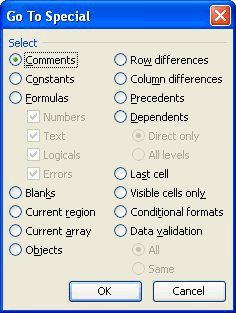
Figure 1. The Go To Special dialog box.

6. Click the Blanks option button, then click OK. All the blank (empty) cells in the selection are selected.
7. Choose Edit | Delete | Shift Cells Up/

The result is that you end up with only the formulas, with the pattern desired.

ExcelTips is your source for cost-effective Microsoft Excel training. This tip (3067) applies to Microsoft Excel 97, 2000, 2002, and 2003.