Please Note: This article is written for users of the following Microsoft Excel versions: 97, 2000, 2002, and 2003. If you are using a later version (Excel 2007 or later), this tip may not work for you. For a version of this tip written specifically for later versions of Excel, click here: Displaying a Hidden First Row.
Written by Allen Wyatt (last updated April 6, 2019)
This tip applies to Excel 97, 2000, 2002, and 2003
Excel makes it easy to hide and unhide rows using the menus. What isn't so easy is displaying a hidden row if that row is above the first visible row in the worksheet. For instance, if you hide rows 1 through 5, Excel will dutifully follow out your instructions. If you later want to unhide any of these rows, the solution isn't so obvious.
To unhide the top rows of a worksheet when they are hidden, follow these steps:
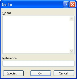
Figure 1. The Go To dialog box.
ExcelTips is your source for cost-effective Microsoft Excel training. This tip (2743) applies to Microsoft Excel 97, 2000, 2002, and 2003. You can find a version of this tip for the ribbon interface of Excel (Excel 2007 and later) here: Displaying a Hidden First Row.

Dive Deep into Macros! Make Excel do things you thought were impossible, discover techniques you won't find anywhere else, and create powerful automated reports. Bill Jelen and Tracy Syrstad help you instantly visualize information to make it actionable. You�ll find step-by-step instructions, real-world case studies, and 50 workbooks packed with examples and solutions. Check out Microsoft Excel 2019 VBA and Macros today!
Don't want to always type the decimal point as you enter information in a worksheet? If you are entering information that ...
Discover MoreOne way to make your worksheets less complex is to get rid of detail and keep only the summary of that detail. Here's how ...
Discover MoreAs you enter data in a worksheet, you may want to have Excel automatically move from cell to cell based on the length of ...
Discover MoreFREE SERVICE: Get tips like this every week in ExcelTips, a free productivity newsletter. Enter your address and click "Subscribe."
2019-04-18 16:46:50
Thomas Papavasileiou
You can also approach the pointer of the mouse in the gray column indicating the row numbers, to the top of the top unhidden row number until it displays a symbol that resembles an equal sign with two arrows, one pointing upwards, starting from the middle of the top horizontal line and the other pointing downwards starting from the middle of the lower horizontal line. When you see that symbol, click and drag downwards, The hidden top row arrears.
An approximate shape of this symbol is as follows
__|__
____
}
Got a version of Excel that uses the menu interface (Excel 97, Excel 2000, Excel 2002, or Excel 2003)? This site is for you! If you use a later version of Excel, visit our ExcelTips site focusing on the ribbon interface.
FREE SERVICE: Get tips like this every week in ExcelTips, a free productivity newsletter. Enter your address and click "Subscribe."
Copyright © 2026 Sharon Parq Associates, Inc.
 Please Note:
This article is written for users of the following Microsoft Excel versions: 97, 2000, 2002, and 2003. If you are using a later version (Excel 2007 or later), this tip may not work for you. For a version of this tip written specifically for later versions of Excel, click here:
Please Note:
This article is written for users of the following Microsoft Excel versions: 97, 2000, 2002, and 2003. If you are using a later version (Excel 2007 or later), this tip may not work for you. For a version of this tip written specifically for later versions of Excel, click here:
Comments