Please Note: This article is written for users of the following Microsoft Excel versions: 97, 2000, 2002, and 2003. If you are using a later version (Excel 2007 or later), this tip may not work for you. For a version of this tip written specifically for later versions of Excel, click here: Displaying a Hidden First Row.
Excel makes it easy to hide and unhide rows using the menus. What isn't so easy is displaying a hidden row if that row is above the first visible row in the worksheet. For instance, if you hide rows 1 through 5, Excel will dutifully follow out your instructions. If you later want to unhide any of these rows, the solution isn't so obvious.
To unhide the top rows of a worksheet when they are hidden, follow these steps:
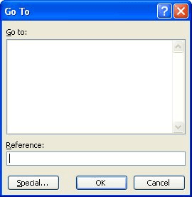
Figure 1. The Go To dialog box.
ExcelTips is your source for cost-effective Microsoft Excel training. This tip (2743) applies to Microsoft Excel 97, 2000, 2002, and 2003. You can find a version of this tip for the ribbon interface of Excel (Excel 2007 and later) here: Displaying a Hidden First Row.

Program Successfully in Excel! This guide will provide you with all the information you need to automate any task in Excel and save time and effort. Learn how to extend Excel's functionality with VBA to create solutions not possible with the standard features. Includes latest information for Excel 2024 and Microsoft 365. Check out Mastering Excel VBA Programming today!
Select a range of cells, and one of those cells will always be the starting point for the range. This tip explains how to ...
Discover MoreGrading in schools is often done using numeric values. However, you may want to change those numeric values into letter ...
Discover MoreYou can edit cell information either in the Formula bar or in the cell itself. Here's how you can configure Excel to ...
Discover MoreFREE SERVICE: Get tips like this every week in ExcelTips, a free productivity newsletter. Enter your address and click "Subscribe."
2019-04-18 16:46:50
Thomas Papavasileiou
You can also approach the pointer of the mouse in the gray column indicating the row numbers, to the top of the top unhidden row number until it displays a symbol that resembles an equal sign with two arrows, one pointing upwards, starting from the middle of the top horizontal line and the other pointing downwards starting from the middle of the lower horizontal line. When you see that symbol, click and drag downwards, The hidden top row arrears.
An approximate shape of this symbol is as follows
__|__
____
}
Got a version of Excel that uses the menu interface (Excel 97, Excel 2000, Excel 2002, or Excel 2003)? This site is for you! If you use a later version of Excel, visit our ExcelTips site focusing on the ribbon interface.
FREE SERVICE: Get tips like this every week in ExcelTips, a free productivity newsletter. Enter your address and click "Subscribe."
Copyright © 2026 Sharon Parq Associates, Inc.
 Please Note:
This article is written for users of the following Microsoft Excel versions: 97, 2000, 2002, and 2003. If you are using a later version (Excel 2007 or later), this tip may not work for you. For a version of this tip written specifically for later versions of Excel, click here:
Please Note:
This article is written for users of the following Microsoft Excel versions: 97, 2000, 2002, and 2003. If you are using a later version (Excel 2007 or later), this tip may not work for you. For a version of this tip written specifically for later versions of Excel, click here:
Comments