Conditionally Highlighting Cells Containing Formulas

You probably already know that you can select all the cells containing formulas in a worksheet by pressing F5 and choosing Special | Formulas. If you need to keep a constant eye on where formulas are located, then repeatedly doing the selecting can get tedious. A better solution is to use the conditional formatting capabilities of Excel to highlight cells with formulas.

Before you can use conditional formatting, however, you need to create a user-defined function that will return True or False, depending on whether there is a formula in a cell. The following macro will do the task very nicely:

Function HasFormula(rCell As Range) As Boolean
    Application.Volatile
    HasFormula = rCell.HasFormula
End Function

To use this with conditional formatting, select the cells you want checked, and then follow these steps:

1. Choose Conditional Formatting from the Format menu. Excel displays the Conditional Formatting dialog box.
2. Make sure the first drop-down list is "Formula Is." (See Figure 1.)



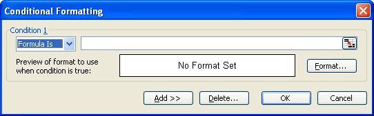
Figure 1. The Conditional Formatting dialog box.

3. In the formula area, enter "=HasFormula(A1)" (without the quote marks). If the active cell in the range that you selected is not A1, you'll need to modify the formula slightly to reflect whatever cell is active.
4. Click the Format button. Excel displays the Format Cells dialog box. (See Figure 2.)



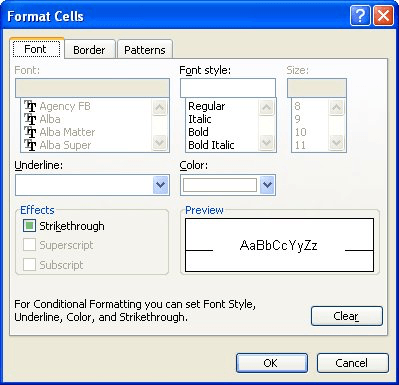
Figure 2. The Format Cells dialog box.

5. Use the controls in the Format Cells dialog box to specify how you want the cells formatted.
6. Click OK to close the Format Cells dialog box.
7. Click OK to close the Conditional Formatting dialog box.

ExcelTips is your source for cost-effective Microsoft Excel training. This tip (3188) applies to Microsoft Excel 97, 2000, 2002, and 2003. You can find a version of this tip for the ribbon interface of Excel (Excel 2007 and later) here: Conditionally Highlighting Cells Containing Formulas.