Displaying Negative Percentages in Red

It's easy using Excel's built-in number formats to display negative values in red. What isn't so obvious is how to display negative percentages in red. This is because Excel doesn't provide a built-in format that addresses this situation.

There are two distinct ways you can display negative percentages in red. One way is to use a custom number format. Precise details on how you put together custom formats has been covered in other issues of ExcelTips, so here is the quick way you can get the desired results:

1. Select the cell (or cells) that may contain negative percentages.
2. Choose Cells from the Format menu. Excel displays the Format Cells dialog box.
3. If the Number tab is not displayed, select it.
4. In the Category list, choose Custom. The dialog box changes so you can enter a custom format. (See Figure 1.)



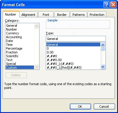
Figure 1. The Number tab of the Format Cells dialog box.

5. In the Type box, enter the following: 0.00%;[Red]-0.00%
6. Click OK.

The format you specify in step 5 displays positive percentages with two decimal places and displays negative percentages in red with two decimal places. (You can modify the number of decimal places in the format, if necessary.)

The other way that you can display negative percentages in red is to use conditional formatting by following these steps:

1. Select the cell (or cells) that may contain negative percentages.
2. Choose Conditional Formatting from the Format menu. Excel displays the Conditional Formatting dialog box.
3. Leave the first drop-down list set to Cell Value Is. (See Figure 2.)



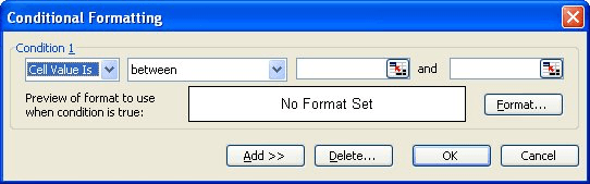
Figure 2. The Conditional Formatting dialog box.

4. Change the second drop-down list to Less Than.
5. In the box to the right of the second drop-down list, enter the numeral 0.
6. Click Format. Excel displays the Format Cells dialog box with the Font tab selected. (See Figure 3.)



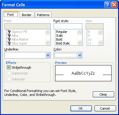
Figure 3. The Font tab of the Format Cells dialog box.

7. Use the Color drop-down list to choose the shade of red you want used for the negative percentages.
8. Click OK to close the Format Cells dialog.
9. Click OK to close the Conditional Formatting dialog.

ExcelTips is your source for cost-effective Microsoft Excel training. This tip (2786) applies to Microsoft Excel 97, 2000, 2002, and 2003. You can find a version of this tip for the ribbon interface of Excel (Excel 2007 and later) here: Displaying Negative Percentages in Red.