Please Note: This article is written for users of the following Microsoft Excel versions: 97, 2000, 2002, and 2003. If you are using a later version (Excel 2007 or later), this tip may not work for you. For a version of this tip written specifically for later versions of Excel, click here: Conditionally Highlighting Cells Containing Formulas.
You probably already know that you can select all the cells containing formulas in a worksheet by pressing F5 and choosing Special | Formulas. If you need to keep a constant eye on where formulas are located, then repeatedly doing the selecting can get tedious. A better solution is to use the conditional formatting capabilities of Excel to highlight cells with formulas.
Before you can use conditional formatting, however, you need to create a user-defined function that will return True or False, depending on whether there is a formula in a cell. The following macro will do the task very nicely:
Function HasFormula(rCell As Range) As Boolean
    Application.Volatile
    HasFormula = rCell.HasFormula
End Function
To use this with conditional formatting, select the cells you want checked, and then follow these steps:
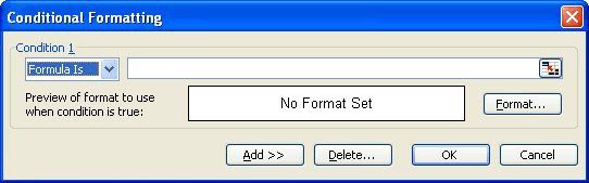
Figure 1. The Conditional Formatting dialog box.
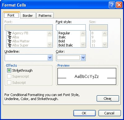
Figure 2. The Format Cells dialog box.
Note:
ExcelTips is your source for cost-effective Microsoft Excel training. This tip (3188) applies to Microsoft Excel 97, 2000, 2002, and 2003. You can find a version of this tip for the ribbon interface of Excel (Excel 2007 and later) here: Conditionally Highlighting Cells Containing Formulas.

Create Custom Apps with VBA! Discover how to extend the capabilities of Office 365 applications with VBA programming. Written in clear terms and understandable language, the book includes systematic tutorials and contains both intermediate and advanced content for experienced VB developers. Designed to be comprehensive, the book addresses not just one Office application, but the entire Office suite. Check out Mastering VBA for Microsoft Office 365 today!
Excel allows you to apply several types of alignments to cells. One type of alignment allows you to indent cell contents ...
Discover MoreExcel provides a variety of underlining styles you can use when you need to underline information within a cell. Here's ...
Discover MoreWhen you format a date in a specific manner, you may be surprised to see that the format changes when you open the ...
Discover MoreFREE SERVICE: Get tips like this every week in ExcelTips, a free productivity newsletter. Enter your address and click "Subscribe."
There are currently no comments for this tip. (Be the first to leave your comment—just use the simple form above!)
Got a version of Excel that uses the menu interface (Excel 97, Excel 2000, Excel 2002, or Excel 2003)? This site is for you! If you use a later version of Excel, visit our ExcelTips site focusing on the ribbon interface.
FREE SERVICE: Get tips like this every week in ExcelTips, a free productivity newsletter. Enter your address and click "Subscribe."
Copyright © 2026 Sharon Parq Associates, Inc.
 Please Note:
This article is written for users of the following Microsoft Excel versions: 97, 2000, 2002, and 2003. If you are using a later version (Excel 2007 or later), this tip may not work for you. For a version of this tip written specifically for later versions of Excel, click here:
Please Note:
This article is written for users of the following Microsoft Excel versions: 97, 2000, 2002, and 2003. If you are using a later version (Excel 2007 or later), this tip may not work for you. For a version of this tip written specifically for later versions of Excel, click here:
Comments