Creating an Amortization Schedule

Written by Allen Wyatt (last updated June 29, 2019)
This tip applies to Excel 97, 2000, 2002, and 2003


Mary would like to use Excel to create an amortization schedule for her home mortgage. Problem is, she doesn't know enough about finance to know which of the financial worksheet functions she should use to do the calculations.

It actually is fairly easy to come up with the right calculations. At its simplest, a mortgage payment consists of two parts: principle and interest. Given some basic information such as how much you are borrowing (your principal), what your interest rate is, and how many monthly payments you need to make, you can then come up with your amortization schedule. Try this out:

  1. Open a blank worksheet.
  2. In cell B1 put your interest rate.
  3. Give cell B1 a name, such as "Rate".
  4. In cell B2 put the number of months you need to pay.
  5. Give cell B2 a name, such as "Term".
  6. In cell B3 put how much you are borrowing.
  7. Give cell B3 a name, such as "Principal".
  8. In cell A6 put the number 1. This represents your payment number.
  9. In cell B6 put this formula: =Principal. The amount you put into cell B3 should now also appear in cell B6.
  10. In cell C6 put this formula: =PPMT(Rate/12,$A6,Term,Principal). This is the amount you will pay toward your principal in this payment. (The PPMT function returns the amount of principle for a given payment.)
  11. In cell D6 put this formula: =IPMT(Rate/12,$A6,Term,Principal). This is the amount you will pay in interest in this payment. (The IPMT function returns the amount of interest for a given payment.)
  12. In cell E6 put this formula: =PMT(Rate/12,Term,Principal). This is the total amount of the payment.
  13. Copy everything from row 6 to row 7.
  14. Change cell A7 to the following formula: =A6+1.
  15. Change cell B7 to the following formula: =B6+C6. This cell now contains the new principal balance for your loan.
  16. Copy row 7 down as many rows as you need.
  17. Add any explanatory labels desired in the ranges A1:A3 and A5:E5. (See Figure 1.)
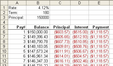
  18. Figure 1. A simple amortization schedule.

Remember that I said that this creates a simple amortization schedule. It doesn't take into account varying interest rates, refinancing, non-monthly payments, additional payments, escrow amounts, or any number of other variables. In such instances you would be better to look for a ready-made amortization template. There are any number of them available online, including these from Microsoft:

http://office.microsoft.com/en-us/templates/TC001056620.aspx

You can also find a very good explanation of amortization schedules at this page:

http://www.tvmcalcs.com/calculators/apps/excel_loan_amortization

ExcelTips is your source for cost-effective Microsoft Excel training. This tip (11627) applies to Microsoft Excel 97, 2000, 2002, and 2003.

Author Bio

Allen Wyatt

With more than 50 non-fiction books and numerous magazine articles to his credit, Allen Wyatt is an internationally recognized author. He is president of Sharon Parq Associates, a computer and publishing services company. ...

MORE FROM ALLEN

Adjusting the Width of Characters

Need to adjust how your characters look horizontally? Word provides an easy way you can scale the horizontal appearance ...

Discover More

Read-Only Documents without a Password

Want to protect your document so it cannot be changed? There are a couple of ways you can do it, and not all of them ...

Discover More

Generating a Count of Word Occurrences

Do you need to know the frequency with which certain words occur in your documents? There is no built-in way to derive ...

Discover More

Dive Deep into Macros! Make Excel do things you thought were impossible, discover techniques you won't find anywhere else, and create powerful automated reports. Bill Jelen and Tracy Syrstad help you instantly visualize information to make it actionable. You’ll find step-by-step instructions, real-world case studies, and 50 workbooks packed with examples and solutions. Check out Microsoft Excel 2019 VBA and Macros today!

More ExcelTips (menu)

Using a Formula to Replace Spaces with Dashes

If you need a formula to change spaces to some other character, the SUBSTITUTE function fits the bill. Here's how to use it.

Discover More

Totaling Across Worksheets

Want to sum the values in the same cell on a range of worksheets? It's not as easy as summing a range on the same ...

Discover More

Finding the Sum of a Sequential Integer Range

In mathematics, the sum of a range of sequential integers, starting with 1, is known as a triangular number or Gaussian ...

Discover More
Subscribe

FREE SERVICE: Get tips like this every week in ExcelTips, a free productivity newsletter. Enter your address and click "Subscribe."

View most recent newsletter.

Comments

If you would like to add an image to your comment (not an avatar, but an image to help in making the point of your comment), include the characters [{fig}] (all 7 characters, in the sequence shown) in your comment text. You’ll be prompted to upload your image when you submit the comment. Maximum image size is 6Mpixels. Images larger than 600px wide or 1000px tall will be reduced. Up to three images may be included in a comment. All images are subject to review. Commenting privileges may be curtailed if inappropriate images are posted.

What is five more than 8?

There are currently no comments for this tip. (Be the first to leave your comment—just use the simple form above!)


This Site

Got a version of Excel that uses the menu interface (Excel 97, Excel 2000, Excel 2002, or Excel 2003)? This site is for you! If you use a later version of Excel, visit our ExcelTips site focusing on the ribbon interface.

Newest Tips
Subscribe

FREE SERVICE: Get tips like this every week in ExcelTips, a free productivity newsletter. Enter your address and click "Subscribe."

(Your e-mail address is not shared with anyone, ever.)

View the most recent newsletter.