Putting a Chart Legend On Its Own Page

Lorna wonders if it is possible to put the legend associated with a chart onto a different page than the chart itself. She is submitting a paper to a journal that wants them separated.

The short answer is that Excel has made the legend and the chart integral to each other and there is not a quick and easy way to separate the two. There is a way to trick Excel into thinking that both elements exist, however. You start to do this may making an additional copy of the chart:

1. Select the chart.
2. Select File | Copy or Ctrl+C. Excel copies the chart.
3. Click in the area you want the legend to appear.
4. Select File | Paste of Ctrl+V. Excel pastes the chart.

You now have two copies of the chart. One will be used for the actual chart (Chart 1) and the other chart (Chart 2) will be the legend. Hiding the legend from Chart 1 is simple and can be accomplished as follows:

1. Single click on the chart.
2. Select Chart | Chart Options. Excel displays the Chart Options dialog box.
3. Click on the Legends tab.
4. Clear the Show Legend check box.
5. Click OK.

The legend no longer appears with the chart. But you have only solved half of the problem. Now you need to work with Chart 2 and isolate the legend on its own page. There are a couple of options to do this.

One option is to use screen capture to obtain a separate image of the legend. For this method, you will need to use a graphics program to trim the image (so it contains just the legend) before placing it back into Excel. Create the chart as usual, then follow these general steps:

1. Use whatever method you prefer to create a screen capture of the legend portion of the chart.
2. Using a graphics program, such as Paint or Adobe Illustrator, trim the image so it contains only the legend.
3. In Excel select Insert | Picture | From File. Excel displays the Insert Picture dialog box.
4. Select the file you created in step 2.
5. Click Insert. The image appears on your worksheet.

At this point, the legend is a simple picture and can be moved to any location you desire.

Another option involves "hiding" the chart so the only visible item in Chart 2 is the legend.

1. Click on Chart 2 so it is selected.
2. Single click on the X-axis line.
3. Select Format | Selected Axis. Excel displays the Format Axis dialog box.
4. Click the Patterns tab. (See Figure 1.)



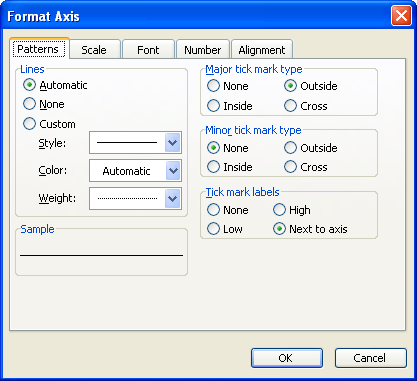
Figure 1. The Patterns tab of the Format Axis dialog box.

5. Select None on all of the options.
6. Click OK. The numbers on the X-axis are removed.
7. Single click on the Y-axis line.
8. Repeat steps 3-5 for the Y-axis.
9. Click OK. The numbers on the Y-axis are removed.
10. Single click on the plot area of the chart.
11. Select Format | Selected Plot Area. Excel displays the Format Plot Area dialog box. (See Figure 2.)



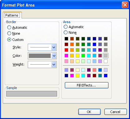
Figure 2. The Format Plot Area dialog box.

12. Select None in the Border and Area sections of the dialog box.
13. Click OK. The border and background of the chart are removed.
14. Single click on one of the horizontal gridlines. Excel selects all of the lines.
15. Select Format | Selected Gridlines. Excel displays the Format Gridlines dialog box. (See Figure 3.)



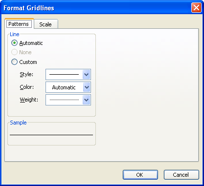
Figure 3. The Format Gridlines dialog box.

16. Select Custom and change the color to white.
17. Click OK. The gridlines are removed and the only remaining portion of the chart is the colored plots.
18. Single click on the plot area.
19. Select Format | Selected Data Series. Excel displays the Format Data Series dialog box. (See Figure 4.)



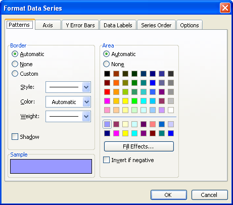
Figure 4. The Format Data Series dialog box.

20. Select None for the Border and Area.
21. Click OK. Excel has "hidden" the chart.

The only element visible at this point is the legend. Keep in mind that the chart is still there, it has just been "hidden" by changing its appearance. This is a long workaround but it gets the job done.

ExcelTips is your source for cost-effective Microsoft Excel training. This tip (8064) applies to Microsoft Excel 97, 2000, 2002, and 2003. You can find a version of this tip for the ribbon interface of Excel (Excel 2007 and later) here: Putting a Chart Legend On Its Own Page.