Please Note: This article is written for users of the following Microsoft Excel versions: 97, 2000, 2002, and 2003. If you are using a later version (Excel 2007 or later), this tip may not work for you. For a version of this tip written specifically for later versions of Excel, click here: Displaying Negative Percentages in Red.
It's easy using Excel's built-in number formats to display negative values in red. What isn't so obvious is how to display negative percentages in red. This is because Excel doesn't provide a built-in format that addresses this situation.
There are two distinct ways you can display negative percentages in red. One way is to use a custom number format. Precise details on how you put together custom formats has been covered in other issues of ExcelTips, so here is the quick way you can get the desired results:
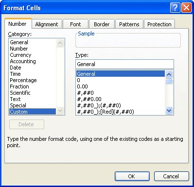
Figure 1. The Number tab of the Format Cells dialog box.
The format you specify in step 5 displays positive percentages with two decimal places and displays negative percentages in red with two decimal places. (You can modify the number of decimal places in the format, if necessary.)
The other way that you can display negative percentages in red is to use conditional formatting by following these steps:
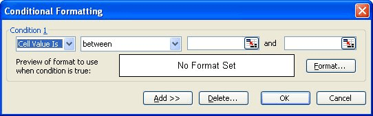
Figure 2. The Conditional Formatting dialog box.
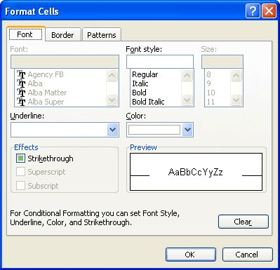
Figure 3. The Font tab of the Format Cells dialog box.
ExcelTips is your source for cost-effective Microsoft Excel training. This tip (2786) applies to Microsoft Excel 97, 2000, 2002, and 2003. You can find a version of this tip for the ribbon interface of Excel (Excel 2007 and later) here: Displaying Negative Percentages in Red.

Best-Selling VBA Tutorial for Beginners Take your Excel knowledge to the next level. With a little background in VBA programming, you can go well beyond basic spreadsheets and functions. Use macros to reduce errors, save time, and integrate with other Microsoft applications. Fully updated for the latest version of Office 365. Check out Microsoft 365 Excel VBA Programming For Dummies today!
Want a quick and easy way to hid the information in a cell? You can do it with a simple three-character custom format.
Discover MoreNeed to cram a bunch of text all on a single line in a cell? You can do it with one of the lesser-known settings in Excel.
Discover MoreIf you are familiar with decimal tabs in Word, you may wonder if you can set the same sort of alignment in Excel. The ...
Discover MoreFREE SERVICE: Get tips like this every week in ExcelTips, a free productivity newsletter. Enter your address and click "Subscribe."
2021-03-22 13:23:32
Alison
Very helpful, thank you!
2019-10-21 13:19:01
Robert C Brewer
Thanks, the explanation was very clear. I used the custom format method with the format: 0.0%;[Red](0.0)%
Got a version of Excel that uses the menu interface (Excel 97, Excel 2000, Excel 2002, or Excel 2003)? This site is for you! If you use a later version of Excel, visit our ExcelTips site focusing on the ribbon interface.
FREE SERVICE: Get tips like this every week in ExcelTips, a free productivity newsletter. Enter your address and click "Subscribe."
Copyright © 2026 Sharon Parq Associates, Inc.
 Please Note:
This article is written for users of the following Microsoft Excel versions: 97, 2000, 2002, and 2003. If you are using a later version (Excel 2007 or later), this tip may not work for you. For a version of this tip written specifically for later versions of Excel, click here:
Please Note:
This article is written for users of the following Microsoft Excel versions: 97, 2000, 2002, and 2003. If you are using a later version (Excel 2007 or later), this tip may not work for you. For a version of this tip written specifically for later versions of Excel, click here:
Comments