Written by Allen Wyatt (last updated September 10, 2022)
This tip applies to Excel 97, 2000, 2002, and 2003
David has a worksheet that he uses to track sales by company over a number of months. The company names are in column A and up to fifteen months of sales are in columns B:P. David would like to create a chart that could be dynamically changed to show the sales for a single company from the worksheet.
There are several ways that this can be done; I'll examine three of them in this tip. For the sake of example, let's assume that the worksheet is named MyData, and that the first row contains data headers. The company names are in the range A2:A151, and the sales data for those companies is in B2:P151.
One approach is to use Excel's AutoFilter capabilities. Create your chart as you normally would, making sure that the chart is configured to draw its data series from the rows of the MyData worksheet. You should also place the chart on its own sheet.
Now, select A1 on MyData and apply an AutoFilter (Data | Filter | AutoFilter). A small drop-down arrow appears at the top of each column. Click the drop-down arrow for column A and select the company you want to view in the chart. Excel redraws the chart to include only the single company.
The only potential drawback to the AutoFilter approach is that each company is considered an independent data series, even though only one of them is displayed in the chart. Because they are independent, each company is charted in a different color. If you want the same charting colors to always be used, then you will need to use one of the other approaches.
Another way to approach the problem is through the use of an "intermediate" data table—one that is created dynamically, pulling only the information you want from the larger data table. The chart is then based on the dynamic intermediate table. Follow these steps:
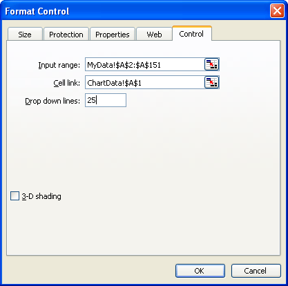
Figure 1. The Format Control dialog box.
=INDEX(MyData!A2:A151,$A$1)
="Data for " & A3
=ChartData!$A$3
You now have a fully functioning dynamic chart. You can use the Combo Box to select a different company, and the chart is redrawn using the data for the company you select. If you want, you can move or copy the Combo Box to the sheet containing your chart so that you can view the updated chart every time you make a selection. You can also, if desired, hide the ChartData worksheet.
A third approach is to use a macro to modify the range on which a chart is based. To prepare for this approach, create two named ranges in your workbook. The first name should be ChartTitle, and it should refer to the formula =OFFSET(MyData!$A$1,22,0,1,1) Click Add, and then define the second name. This one should be called ChartXRange, and it should refer to the formula =OFFSET(MyData!$A$1,22,0,1,15). (See Figure 2.)
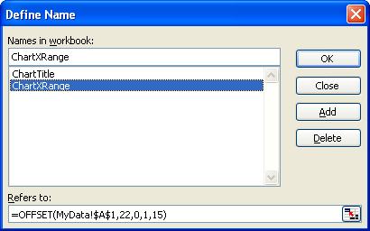
Figure 2. The Define Name dialog box.
With the names defined, you can select the range MyData!B1:P2 and create your chart. You should base the chart on this simple range, and make sure that you place some temporary text in the chart title. Make sure the chart is created on its own sheet and that you name the sheet ChartSheet.
With the chart created, right-click the chart and choose Source Data. Excel displays the Source Data dialog box, and you should choose the Series tab. Since you based the chart on the headers and a single row of data, there should be a single data series in the dialog box. Replace whatever is in the Values box with the following formula:
='Book1'!ChartXRange
Make sure you replace Book1 with the name of the workbook in which you are working. Click OK, and the chart is now based on the named range you specified earlier. You can now select the chart title and place the following in the Formula bar to make the title dynamic:
=MyData!ChartTitle
Now you are ready to add the macro that makes everything dynamic. Display the VBA Editor and add the following macro to the code window for the MyData worksheet. (Double-click the worksheet name in the Project Explorer area.)
Private Sub Worksheet_BeforeDoubleClick(ByVal Target As Excel.Range, Cancel As Boolean)
    ActiveWorkbook.Names.Add Name:="ChartXRange", _
        RefersToR1C1:="=OFFSET(MyData!R1C1," & _
            ActiveCell.Row - 1 & ",1,1,15)"
    ActiveWorkbook.Names.Add Name:="ChartTitle", _
        RefersToR1C1:="=OFFSET(MyData!R1C1," & _
            ActiveCell.Row - 1 & ",0,1,1)"
    Sheets("ChartSheet").Activate
    Cancel = True
End Sub
Now you can display the MyData worksheet and double-click any row. (Well, double-click in column A for a row.) The macro then updates the named ranges so that they point to the row on which you double-clicked, and then displays the ChartSheet sheet. The chart (and title) are redrawn to reflect the data in the row on which you double-clicked.
ExcelTips is your source for cost-effective Microsoft Excel training. This tip (2377) applies to Microsoft Excel 97, 2000, 2002, and 2003.

Excel Smarts for Beginners! Featuring the friendly and trusted For Dummies style, this popular guide shows beginners how to get up and running with Excel while also helping more experienced users get comfortable with the newest features. Check out Excel 2019 For Dummies today!
Want a handy way to make the data ranges for your chart more dynamic? Here are some great ideas you can put to work right ...
Discover MoreUnhappy with the default size that Excel uses for embedded chart objects? You can't change the size at which they are ...
Discover MoreWhen creating a chart from information that contains empty cells, you can direct Excel how it should proceed. This tip ...
Discover MoreFREE SERVICE: Get tips like this every week in ExcelTips, a free productivity newsletter. Enter your address and click "Subscribe."
2022-12-16 20:13:39
Venetia
Dear Allan
I have found your tips very helpful. RE: Automatically Creating Charts for Individual Rows in a Data Table
I teach and I am trying to create charts for each student following a final exam, so this page has been very helpful. But I have over 100 students.
I love solution 2 for what I am trying to do. However, all the names do not show in the choice box. Is there a way that gives me a scrolling drop down list for this solution.
Got a version of Excel that uses the menu interface (Excel 97, Excel 2000, Excel 2002, or Excel 2003)? This site is for you! If you use a later version of Excel, visit our ExcelTips site focusing on the ribbon interface.
FREE SERVICE: Get tips like this every week in ExcelTips, a free productivity newsletter. Enter your address and click "Subscribe."
Copyright © 2026 Sharon Parq Associates, Inc.
Comments