Relative References within Named Ranges

Chris has set up a worksheet where he uses named ranges (rows) in his formulas. He has named the entire sales row as "Sales," and then uses the Sales name in various formulas. For instance, in any given column he can say =Sales, and the value of the Sales row, for that column, is returned by the formula. Chris was wondering how to use the same formula technique to refer to cells in different columns.

There are a couple of different ways this can be done. First of all, you can use the INDEX function to refer to the cells. The rigorous way to refer to the value of Sales in the same column is as follows:

=INDEX(Sales,1,COLUMN())

This works if the Sales named range really does refer to the entire row in the worksheet. If it does not (for instance, Sales may refer to cells C10:K10), then the following formula refers to the value of Sales in the same column in which the formula occurs:

=INDEX(Sales,1,COLUMN()-COLUMN(Sales)+1)

If you want to refer to a different column, then simply adjust the value that is added to the column designation in the INDEX function. For example, if you wanted to determine the difference between the sales for the current column and the sales in the previous column, then you would use the following:

=INDEX(Sales,1,COLUMN()-COLUMN(Sales)+1) - INDEX(Sales,1,COLUMN()-COLUMN(Sales))

The "shorthand" version for this formula would be as follows:

=Sales - INDEX(Sales,1,COLUMN()-COLUMN(Sales))

There are other functions you can use besides INDEX (such as OFFSET), but the technique is still the same—you must find a way to refer to an offset from the present column.

There is an easier way to get at the desired data, however. Let's say that your Sales range also has a heading row about it, similar to what is shown in the following: (See Figure 1.)

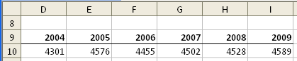
Figure 1. Example sales data.

The heading row lists the years for the range, and the values under the headings are those that actually make up the Sales range. To make sure this technique will work, follow these steps:

1. Choose Options from the Tools menu. Excel displays the Options dialog box.
2. Make sure the Calculation tab is displayed. (See Figure 2.)



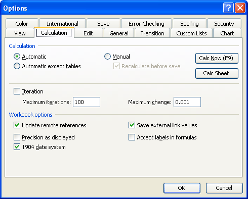
Figure 2. The Calculation tab of the Options dialog box.

3. Ensure that the Accept Labels in Formulas check box is selected.
4. Click OK.

With this configuration change done, you can use the following as your formulas:

=Sales '2009' – Sales '2004'

What you are actually doing is instructing Excel to work with unions of cells. In this instance, Sales '2009' returns the cell at the intersection of the Sales range and the '2009' column. A similar union is returned for the portion of the formula to the right of the minus sign. The result is the subtraction of the two values you wanted.

ExcelTips is your source for cost-effective Microsoft Excel training. This tip (3202) applies to Microsoft Excel 97, 2000, 2002, and 2003. You can find a version of this tip for the ribbon interface of Excel (Excel 2007 and later) here: Relative References within Named Ranges.