Please Note: This article is written for users of the following Microsoft Excel versions: 97, 2000, 2002, and 2003. If you are using a later version (Excel 2007 or later), this tip may not work for you. For a version of this tip written specifically for later versions of Excel, click here: Using Graphics to Represent Data Series.
Excel is great at creating all sorts of charts from your data. You can even customize the charts to your heart's content. One of the customizations you can make is to replace the regular bars (in a bar chart) with your own graphics. For instance, you might have a small graphic of a house that you want to use for the bars. This could be great if you wanted to used "stacked" houses to represent, for instance, housing starts in an area.
To use your own graphics in place of Excel's built-in bars, follow these steps:
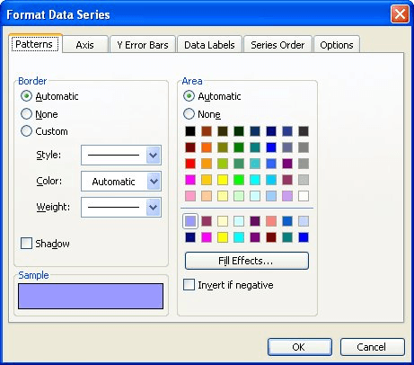
Figure 1. The Patterns tab of the Format Data Series dialog box.
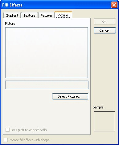
Figure 2. The Picture tab from the Fill Effects dialog box.
ExcelTips is your source for cost-effective Microsoft Excel training. This tip (3199) applies to Microsoft Excel 97, 2000, 2002, and 2003. You can find a version of this tip for the ribbon interface of Excel (Excel 2007 and later) here: Using Graphics to Represent Data Series.

Best-Selling VBA Tutorial for Beginners Take your Excel knowledge to the next level. With a little background in VBA programming, you can go well beyond basic spreadsheets and functions. Use macros to reduce errors, save time, and integrate with other Microsoft applications. Fully updated for the latest version of Office 365. Check out Microsoft 365 Excel VBA Programming For Dummies today!
Using the copy and paste techniques you already know, you can copy and paste drawing objects. In this way, you can ...
Discover MoreAutoShapes can easily contain text—just click on the shape and start typing away. You may want the text in the ...
Discover MoreIf you add callouts using the drawing tools in Excel, you may have noticed that they don't always stay where you expect ...
Discover MoreFREE SERVICE: Get tips like this every week in ExcelTips, a free productivity newsletter. Enter your address and click "Subscribe."
There are currently no comments for this tip. (Be the first to leave your comment—just use the simple form above!)
Got a version of Excel that uses the menu interface (Excel 97, Excel 2000, Excel 2002, or Excel 2003)? This site is for you! If you use a later version of Excel, visit our ExcelTips site focusing on the ribbon interface.
FREE SERVICE: Get tips like this every week in ExcelTips, a free productivity newsletter. Enter your address and click "Subscribe."
Copyright © 2026 Sharon Parq Associates, Inc.
 Please Note:
This article is written for users of the following Microsoft Excel versions: 97, 2000, 2002, and 2003. If you are using a later version (Excel 2007 or later), this tip may not work for you. For a version of this tip written specifically for later versions of Excel, click here:
Please Note:
This article is written for users of the following Microsoft Excel versions: 97, 2000, 2002, and 2003. If you are using a later version (Excel 2007 or later), this tip may not work for you. For a version of this tip written specifically for later versions of Excel, click here:
Comments