Please Note: This article is written for users of the following Microsoft Excel versions: 97, 2000, 2002, and 2003. If you are using a later version (Excel 2007 or later), this tip may not work for you. For a version of this tip written specifically for later versions of Excel, click here: Automatic Lines for Dividing Lists.
Let's say you have a list of company transactions. Each transaction includes a department number, a title, and other information (amount, date, time, sales rep, etc.). As you get more and more of these items in your list, you may want a way to automatically add "dividing lines" based on the department number. For instance, when the department number changes, you may want to include a line between the two departments.
To add this type of formatting to your list, start by sorting your data table by department. Then follow these steps:
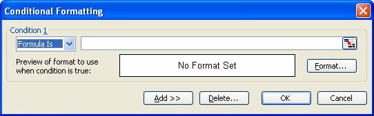
Figure 1. The Conditional Formatting dialog box.
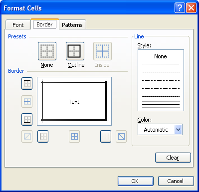
Figure 2. The Borders tab of the Format Cells dialog box.
That's it; you should now see a line that appears across the entire width of your data every time the department changes.
ExcelTips is your source for cost-effective Microsoft Excel training. This tip (3189) applies to Microsoft Excel 97, 2000, 2002, and 2003. You can find a version of this tip for the ribbon interface of Excel (Excel 2007 and later) here: Automatic Lines for Dividing Lists.

Best-Selling VBA Tutorial for Beginners Take your Excel knowledge to the next level. With a little background in VBA programming, you can go well beyond basic spreadsheets and functions. Use macros to reduce errors, save time, and integrate with other Microsoft applications. Fully updated for the latest version of Office 365. Check out Microsoft 365 Excel VBA Programming For Dummies today!
Want a quick way to replace background colors in cells? It's easy to do using Find and Replace, or you can simply use the ...
Discover MoreExcel provides a variety of tools you can use to make your data look more presentable on the screen and on a printout. ...
Discover MoreNeed to get rid of the borders around a cell? The shortcut in this tip can make quick work of this formatting task.
Discover MoreFREE SERVICE: Get tips like this every week in ExcelTips, a free productivity newsletter. Enter your address and click "Subscribe."
There are currently no comments for this tip. (Be the first to leave your comment—just use the simple form above!)
Got a version of Excel that uses the menu interface (Excel 97, Excel 2000, Excel 2002, or Excel 2003)? This site is for you! If you use a later version of Excel, visit our ExcelTips site focusing on the ribbon interface.
FREE SERVICE: Get tips like this every week in ExcelTips, a free productivity newsletter. Enter your address and click "Subscribe."
Copyright © 2026 Sharon Parq Associates, Inc.
 Please Note:
This article is written for users of the following Microsoft Excel versions: 97, 2000, 2002, and 2003. If you are using a later version (Excel 2007 or later), this tip may not work for you. For a version of this tip written specifically for later versions of Excel, click here:
Please Note:
This article is written for users of the following Microsoft Excel versions: 97, 2000, 2002, and 2003. If you are using a later version (Excel 2007 or later), this tip may not work for you. For a version of this tip written specifically for later versions of Excel, click here:
Comments