Please Note: This article is written for users of the following Microsoft Excel versions: 97, 2000, 2002, and 2003. If you are using a later version (Excel 2007 or later), this tip may not work for you. For a version of this tip written specifically for later versions of Excel, click here: AutoFilling with the Alphabet.
Written by Allen Wyatt (last updated April 4, 2020)
This tip applies to Excel 97, 2000, 2002, and 2003
Marlene is a teacher and she has students who love word searches. She finds it quite time consuming to make them, but the students seem to remember the course material much better when she uses them. Marlene wondered if there was some way to AutoFill a range of cells with letters of the alphabet, A through Z. That way she can use the feature to fill in the squares of the word search with letters, before she replaces some of those letters with the actual words to be searched.
The AutoFill tool in Excel has a few standard sequences it will fill automatically, such as dates and numeric sequences. The very powerful part of AutoFill, however, is that you can create custom lists that the tool uses just as easily as the built-in sequences. In order to create a custom list manually, you can follow these steps:
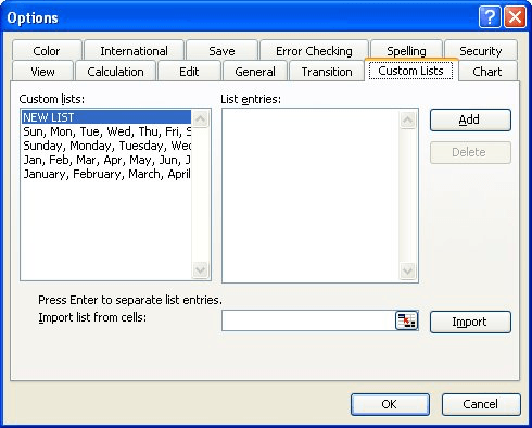
Figure 1. The Custom Lists tab of the Options dialog box.
You've now created your custom list, and you can close any open dialog boxes. To use the custom list, just type one or two letters you want to start the sequence with, select those cells, and use the AutoFill handle to drag over as many cells as you want to fill.
There's another way to create the custom list that may be a bit easier, just in case you don't want to type twenty-six letters in the dialog box. Instead, if you already have the letters of the alphabet in twenty-six cells, simply select those cells and follow these steps:
Now you can close the dialog box and use the custom list as you desire.
Of course, there is one drawback with using a custom list, especially when it comes to creating word searches: the letters added to blank squares are always in a predictable sequence, which could make finding the actual words a bit easier than you want. To make the puzzles a bit more challenging, it would be better to fill the non-word squares with random letters.
One easy way to get random letters is to use the following formula:
=CHAR(RANDBETWEEN(65,90))
This formula works because the RANDBETWEEN function returns a random numeric value between the two boundary values provided. In this case, it will return a value between 65 and 90, which are the ASCII values of the letters A and Z, respectively. The CHAR function is then used to convert this random numeric value into an actual letter.
The RANDBETWEEN function is part of the Analysis ToolPak, an add-in which many people have installed in Excel. (Choose Tools | Add-ins to see if you have it installed.) If you prefer to not have the add-in enabled, then you can rely upon a more basic formula, such as the following:
=CHAR((65+(90-65)*RAND()))
The CHAR function should look familiar; the only difference is the use of the RAND function to generate the random value instead of RANDBETWEEN.
If you create a lot of word search puzzles, then you may want to use a macro to fill a range of cells with random letters of the alphabet. There are any number of ways that such a macro could be put together; the following is one that is particularly flexible. It will work with either a pre-selected range (a range selected when you run the macro) or you can select a range after you run the macro.
Sub AlphaFill()
    Dim Cell, CellChars
    Dim Default, Prompt, Title
    Dim rangeSelected As Range
    Dim UpperCase As Boolean

    Title = "AlphaFill Cell Selection"
    Default = Selection.Address
    Prompt = vbCrLf _
      & "Use mouse in conjunction with " _
      & "SHIFT and CTRL keys to" & vbCrLf _
      & "click and drag or type in name(s) " _
      & "of cell(s) to AlphaFill" & vbCrLf & vbCrLf _
      & "Currently selected cell(s): "
      & Selection.Address

    On Error Resume Next
    Set rangeSelected = InputBox(Prompt, Title, _
      Default, Type:=8)
    If rangeSelected Is Nothing Then Exit Sub

    UpperCase = True
    Randomize
    For Each Cell In rangeSelected
        CellChars = Chr(64 + Int((Rnd * 26) + 1))
        If Not UpperCase Then CellChars = LCase(CellChars)
        Cell.Value = CellChars
    Next
End Sub
The macro code, as written, inserts the uppercase letters into whatever range you specify. If you want to use lowercase letters instead, then all you need to do is set the UpperCase variable to False rather than True.
Note:
ExcelTips is your source for cost-effective Microsoft Excel training. This tip (3109) applies to Microsoft Excel 97, 2000, 2002, and 2003. You can find a version of this tip for the ribbon interface of Excel (Excel 2007 and later) here: AutoFilling with the Alphabet.

Professional Development Guidance! Four world-class developers offer start-to-finish guidance for building powerful, robust, and secure applications with Excel. The authors show how to consistently make the right design decisions and make the most of Excel's powerful features. Check out Professional Excel Development today!
The AutoFill feature can be used for more than just incrementing information into cells. This tip explains how to access ...
Discover MoreUsing the fill handle is a great way to quickly fill a range of cells with values. Sometimes, however, the way to fill ...
Discover MoreNeed to fill a range of cells with the days of the week? Excel makes it easy to do so using AutoFill.
Discover MoreFREE SERVICE: Get tips like this every week in ExcelTips, a free productivity newsletter. Enter your address and click "Subscribe."
There are currently no comments for this tip. (Be the first to leave your comment—just use the simple form above!)
Got a version of Excel that uses the menu interface (Excel 97, Excel 2000, Excel 2002, or Excel 2003)? This site is for you! If you use a later version of Excel, visit our ExcelTips site focusing on the ribbon interface.
FREE SERVICE: Get tips like this every week in ExcelTips, a free productivity newsletter. Enter your address and click "Subscribe."
Copyright © 2026 Sharon Parq Associates, Inc.
 Please Note:
This article is written for users of the following Microsoft Excel versions: 97, 2000, 2002, and 2003. If you are using a later version (Excel 2007 or later), this tip may not work for you. For a version of this tip written specifically for later versions of Excel, click here:
Please Note:
This article is written for users of the following Microsoft Excel versions: 97, 2000, 2002, and 2003. If you are using a later version (Excel 2007 or later), this tip may not work for you. For a version of this tip written specifically for later versions of Excel, click here:
Comments