Please Note: This article is written for users of the following Microsoft Excel versions: 97, 2000, 2002, and 2003. If you are using a later version (Excel 2007 or later), this tip may not work for you. For a version of this tip written specifically for later versions of Excel, click here: Performing Calculations while Filtering.
Filtering a list means displaying only a part of it. You provide the criteria you want used, and then Excel displays only those list records that match the criteria. Filtering is especially useful if you have a large list and you want to work with only a subset of the records in the list. Other ExcelTips have described different ways you can create and apply filters to your worksheets.
When you are using the advanced filtering capabilities of Excel you can perform calculations during the filtering process. For instance, let's assume you have a large inventory list in a worksheet, and you want to filter the list to show only those records that were in a particular department and that have a higher-than-average profit. The inventory is contained in starts at cell A6 (with your column headings) and the profit is listed in column I. (See Figure 1.)
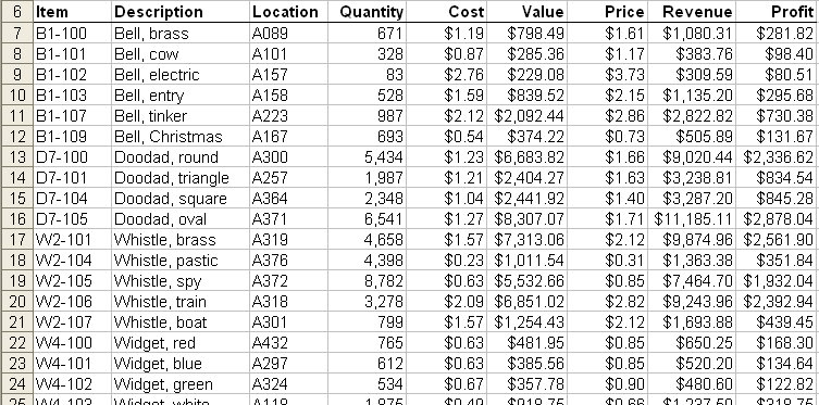
Figure 1. Example inventory data in a worksheet.
You can use an advanced filter by setting up your criteria in other cells. For instance, let's say that your criteria are in the cell range A1:B2. (See Figure 2.)
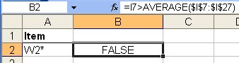
Figure 2. Example filtering criteria.
Row 1 contains the names of the columns in your datasheet that you want compared in the filtering. Thus, cell A1 contains the name "Item" because you want the value under it (in cell A2) to be used in filtering the data table based on the contents of the Item column. There is no column name in cell B1 because you aren't keying the criteria on a column's contents; you want it based on a calculation. Here are the formulas you should place in cells A2 and B2:
| Cell | Formula | |
|---|---|---|
| A2 | ="W2*" | |
| B2 | =I7>AVERAGE($I$7:$I$42) |
This example provides for a text comparison related to the department number (in cell A2) and a comparison of the profit for the item (I7, which is a relative cell reference and therefore changes for each comparison) to the average profit for the entire inventory ($I$7:$I$42, which is an absolute reference and therefore does not change for each comparison). If an absolute reference had not been used for the AVERAGE function, the wrong results would have been generated by the filtering.
When you apply an advanced filter to your inventory data (as described in other ExcelTips), the result, using the above criteria, is that only those records that had a profit greater than the average (the average in I7:I42) were displayed.
ExcelTips is your source for cost-effective Microsoft Excel training. This tip (2982) applies to Microsoft Excel 97, 2000, 2002, and 2003. You can find a version of this tip for the ribbon interface of Excel (Excel 2007 and later) here: Performing Calculations while Filtering.

Best-Selling VBA Tutorial for Beginners Take your Excel knowledge to the next level. With a little background in VBA programming, you can go well beyond basic spreadsheets and functions. Use macros to reduce errors, save time, and integrate with other Microsoft applications. Fully updated for the latest version of Office 365. Check out Microsoft 365 Excel VBA Programming For Dummies today!
When working with large amounts of data, you may have a need to extract just the information that meets the criteria you ...
Discover MoreThe advanced filtering feature in Excel allows you to quickly copy unique information from one data list to another. If ...
Discover MoreFiltering is a great asset when you need to get a handle on a subset of your data. Excel even makes it easy to copy the ...
Discover MoreFREE SERVICE: Get tips like this every week in ExcelTips, a free productivity newsletter. Enter your address and click "Subscribe."
There are currently no comments for this tip. (Be the first to leave your comment—just use the simple form above!)
Got a version of Excel that uses the menu interface (Excel 97, Excel 2000, Excel 2002, or Excel 2003)? This site is for you! If you use a later version of Excel, visit our ExcelTips site focusing on the ribbon interface.
FREE SERVICE: Get tips like this every week in ExcelTips, a free productivity newsletter. Enter your address and click "Subscribe."
Copyright © 2026 Sharon Parq Associates, Inc.
 Please Note:
This article is written for users of the following Microsoft Excel versions: 97, 2000, 2002, and 2003. If you are using a later version (Excel 2007 or later), this tip may not work for you. For a version of this tip written specifically for later versions of Excel, click here:
Please Note:
This article is written for users of the following Microsoft Excel versions: 97, 2000, 2002, and 2003. If you are using a later version (Excel 2007 or later), this tip may not work for you. For a version of this tip written specifically for later versions of Excel, click here:
Comments