Creating Dependent Drop-Lists

Carol asked if there is a way in Excel to create drop-down lists so that the second drop-down list is dependent on the selection made in the first drop-down list.

There are actually a number of different ways you can accomplish this task, ranging from simple formulas to complex macros. The method you choose depends, most directly, on the type of drop-down lists you want to create. There are actually three types of drop-down lists you can create in Excel:

• Validation lists. If you want to limit input in certain cells, then you can create drop-down validation lists.
• Forms lists. You can use the Forms toolbar (View | Toolbars | Forms) to create drop-down lists. These are great if you are going to create a protected Excel form.
• Userforms. These are dialog boxes, created in the VBA editor. You "run" a userform by calling it from a macro. This is the most versatile form of user interface, as it allows you the greatest latitude in what the user sees. (It also requires the most advanced knowledge of Excel in order to create.)

Rather than discuss how to create dependent drop-lists based on each of these types of drop-down lists, I'll choose to examine the simplest method, which will suffice for most people. If you use the INDIRECT function along with data validation lists, it is quite easy to get the result you want:

1. On a blank worksheet in your workbook, create a list of the items that will be in the first drop-down list. For instance, create a list of departments in your company, such as Sales, Research, Executive, Production, etc. (These should be single-word entries in the list.)
2. Select the list of items you created in step 1 and name the range using a name such as "Departments."
3. On the same worksheet, create a list of items that could appear in the secondary drop-down list. There should be one list for each entry in the list you made in step 1. For instance, you could create a list of Sales personnel, a list of Research personnel, etc.
4. List by list, select the lists you created in step 3. Give each list a single-word name that matches the names used in the list in step 1, i.e., Sales, Research, Executive, etc.
5. Switch to the worksheet where you want to have the drop-down lists appear.
6. Select the cells where users should be able to enter items from your first list—the one created in step 1.
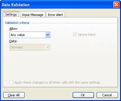
7. Choose Validation from the Data menu. Excel displays the Data Validation dialog box. (See Figure 1.)



Figure 1. The Data Validation dialog box.

8. Using the Allow drop-down list, choose List.
9. In the Source box, enter an equal sign followed by the name you created in step 2. For instance, =Departments.
10. Click OK. You have now specified that only information from your first list can be entered into the cells you selected in step 6.
11. Select the cells where users should be able to enter items from the dependent lists. For instance, select the cells just to the right of the cells you selected in step 6.
12. Choose Validation from the Data menu. Excel displays the Data Validation dialog box.
13. Using the Allow drop-down list, choose List.
14. In the Source box, enter a formula that uses the INDIRECT function. If the first cell of the range selected in step 11 is cell B3, and you want that first cell to be dependent on what is chosen in cell A3, then you would use the following formula:

     =INDIRECT(A3)

15. Click OK.

That's it. Now people can only select from your major list if they are using one of the cells specified in step 6, and from the appropriate dependent lists if they choose one of the cells in step 11.

There are lots of different variations of this approach (using data validation). You can find more information on some of these approaches by visiting these Web pages:

http://www.ozgrid.com/download/ (download the MatchingLists.zip file)
http://www.contextures.com/xlDataVal02.html

ExcelTips is your source for cost-effective Microsoft Excel training. This tip (2972) applies to Microsoft Excel 97, 2000, 2002, and 2003. You can find a version of this tip for the ribbon interface of Excel (Excel 2007 and later) here: Creating Dependent Drop-Lists.