Counting Records Matching Multiple Criteria

It is not unusual to use Excel to create small databases. For instance, you might keep a list of your poodle-breeders club members in Excel, or you might use it to maintain a list of your active sales contacts. In those instances, you might wonder how you could get a count of the number of records that meet more than one criteria.

Let's say that you are analyzing your membership list, and you wanted to determine a count of the records in which the gender column contains "F" and the city column contains a particular city, such as "Norwood". This, of course, would be helpful because it would answer the burning question of how many female members of your group live in Norwood.

Excel includes a number of worksheet functions that are handy for determining the count of records in a list. How you can use these in a situation where two criteria must be met may not be immediately obvious. Let's examine five specific ways you can achieve the desired goal of female members from Norwood. (Assume that column B is the gender column and column H is the city column.)

The first way to solve the problem is through the use of the DCOUNTA function. This function allows you to define a set of criteria, and use those criteria as the basis for analyzing a list of data. Like all the data functions in Excel, DCOUNTA relies upon three parameters: the data range, the column to use in the comparisons, and the criteria range. To use the function, set up a criteria table in an unused area of your worksheet. For instance, you could set up the following in cells AA1 through AB2:

Then, assuming your original data table is in cells A1:K500 (obviously a large poodle breeders' club), then you could use the following to determine the count:

=DCOUNTA(A1:K500,1,AA1:AB2)

The result is a count that meets the criteria you specified in AA1:AB2. Note, as well, that the names you used in AA1 and AB1 must exactly match the labels you used in your table records. When they do, the contents of the Gender column (column B) must be F and the contents of the City column (column H) must be Norwood in order for the record to be added to the count.

The second solution is to use an array formula to return a single answer. The array formula interestingly uses the SUM function and a little bit of Boolean arithmetic to determine if a record should be counted. Consider the following:

=SUM((B2:B500="F")*(H2:H500="Norwood"))

Simply type the above formula in a cell and then finish it by pressing Ctrl+Shift+Enter; this lets Excel know you are entering an array formula. The formula works because it compares the contents of each row in the array, in turn, according to the criteria specified in the formula. It first compares the contents of the B column with "F"; if it matches, then the comparison returns True, which is the numeric value 1. The contents of column F are then compared to "Norwood". If that comparison is true, then 1 is returned. Thus, 1 * 1 would equal 1, and this is added to the SUM of the array. If either comparison is False, then the numeric value 0 is returned, and 1 * 0 equals 0 (as does 0 * 0 and 0 * 1), which doesn't affect the running SUM.

A third and closely related approach is to use the SUMPRODUCT function, but not in an array formula. You could simply use the following in any cell where you wanted to know if the two criteria are met:

SUMPRODUCT((B2:B500="F")*(H2:H500="Norwood"))

Remember, this is not an array formula, so you don't need to press Ctrl+Shift+Enter. The formula works, again, through the magic of Boolean math.

A fourth possible solution, which is a bit more manual than those discussed already, is to use the AutoFilter feature along with a subtotal. Assuming your data records are in A1:K500, with column labels in row 1, you would follow these steps:

1. Select any cell in the data table.
2. Choose Filter from the Data menu, then choose AutoFilter. Excel should display the AutoFilter drop-down indicators next to each column label in row 1.
3. Using the drop-down indicator for the gender column (column B), choose F. Your list is automatically filtered to only display female members.
4. Using the drop-down indicator for the city column (column H), choose Norwood. Your list is automatically displayed to only display female members living in Norwood.
5. At the bottom of the data table (row 501), in any column desired, enter the following formula:

=SUBTOTAL(3,B2:B500)

This formula causes the SUBTOTAL function to apply the COUNTA function to derive a subtotal. In other words, it returns a count of all records that are displayed by the filtering; this is the count desired.

A fifth approach is to use the Conditional Sum Wizard to come up with a formula for you. (The Conditional Sum Wizard is available as an Excel add-in. Choose Tools | Add-Ins to make sure that the wizard is installed and available.) Follow these steps to use the Conditional Sum Wizard:

1. Select a cell somewhere within the data you want to analyze.
2. Choose Conditional Sum from the Tools menu. Excel displays the first step of the Conditional Sum Wizard. The full range of your data should already be shown in the dialog box. (See Figure 1.)



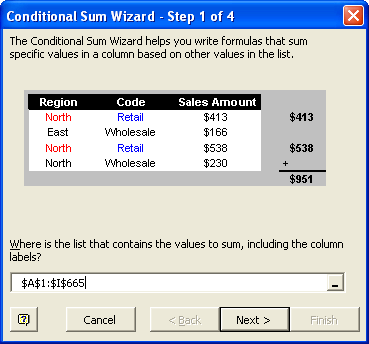
Figure 1. The Conditional Sum Wizard.

3. Click on Next. Excel displays the next step of the wizard.
4. In the Column to Sum drop-down list, choose Gender.
5. In the Column drop-down, choose Gender.
6. In the Is drop-down, choose the equal sign.
7. In the This Value drop-down, choose F.
8. Click on Add. The condition you specified now appears in the dialog box.
9. In the Column drop-down, choose City.
10. In the Is drop-down, choose the equal sign.
11. In the This Value drop-down, choose Norwood.
12. Click on Add. The second condition now appears in the dialog box.
13. Click on Next. Excel displays the third step of the wizard.
14. Choose Copy Just the Formula To a Single Cell.
15. Click on Next. Excel displays the fourth (and final) step of the wizard.
16. In the worksheet, click on the cell you want to contain the result of your formula.
17. Click on Finish.

The result is a formula, appropriate for the conditions you specified, in the cell you selected in step 1.

There are undoubtedly countless other possible solutions you could use to figure out the count of records. These, however, are the "pick of the lot," and allow you to determine the answer quickly and easily.

ExcelTips is your source for cost-effective Microsoft Excel training. This tip (2809) applies to Microsoft Excel 97, 2000, 2002, and 2003. You can find a version of this tip for the ribbon interface of Excel (Excel 2007 and later) here: Counting Records Matching Multiple Criteria.