Please Note: This article is written for users of the following Microsoft Excel versions: 97, 2000, 2002, and 2003. If you are using a later version (Excel 2007 or later), this tip may not work for you. For a version of this tip written specifically for later versions of Excel, click here: Conditionally Formatting an Entire Row.
Written by Allen Wyatt (last updated April 11, 2020)
This tip applies to Excel 97, 2000, 2002, and 2003
Graham described a problem he was having with a worksheet. He wanted to use conditional formatting to highlight all the cells in a row, if the value in column E was greater than a particular value. He was having problems coming up with the proper way to do that.
Suppose for a moment that your data is in cells A3:H50. You can apply the proper conditional formatting by following these steps:
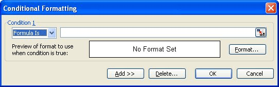
Figure 1. The Conditional Formatting dialog box.
=$E3>40000
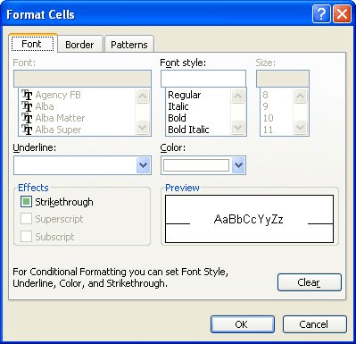
Figure 2. The Format Cells dialog box.
This formula used in the conditional format works because you use the absolute indicator (the dollar sign) just before the column letter. Any reference that has the $ before it is not changed when Excel propagates it throughout a range. In this case, the cell reference will always be to column E, although the row portion of the reference can change.
ExcelTips is your source for cost-effective Microsoft Excel training. This tip (2798) applies to Microsoft Excel 97, 2000, 2002, and 2003. You can find a version of this tip for the ribbon interface of Excel (Excel 2007 and later) here: Conditionally Formatting an Entire Row.

Dive Deep into Macros! Make Excel do things you thought were impossible, discover techniques you won't find anywhere else, and create powerful automated reports. Bill Jelen and Tracy Syrstad help you instantly visualize information to make it actionable. You�ll find step-by-step instructions, real-world case studies, and 50 workbooks packed with examples and solutions. Check out Microsoft Excel 2019 VBA and Macros today!
When entering data in a worksheet, Excel tries to figure out how your entry can best be shown on the screen. When it ...
Discover MoreWhen creating custom formats, you can employ a wide range of codes to define your formatting pattern. This tip focuses on ...
Discover MoreHave you ever been using a workbook, only to open it one day and find that Excel has changed the height of your rows or ...
Discover MoreFREE SERVICE: Get tips like this every week in ExcelTips, a free productivity newsletter. Enter your address and click "Subscribe."
There are currently no comments for this tip. (Be the first to leave your comment—just use the simple form above!)
Got a version of Excel that uses the menu interface (Excel 97, Excel 2000, Excel 2002, or Excel 2003)? This site is for you! If you use a later version of Excel, visit our ExcelTips site focusing on the ribbon interface.
FREE SERVICE: Get tips like this every week in ExcelTips, a free productivity newsletter. Enter your address and click "Subscribe."
Copyright © 2026 Sharon Parq Associates, Inc.
 Please Note:
This article is written for users of the following Microsoft Excel versions: 97, 2000, 2002, and 2003. If you are using a later version (Excel 2007 or later), this tip may not work for you. For a version of this tip written specifically for later versions of Excel, click here:
Please Note:
This article is written for users of the following Microsoft Excel versions: 97, 2000, 2002, and 2003. If you are using a later version (Excel 2007 or later), this tip may not work for you. For a version of this tip written specifically for later versions of Excel, click here:
Comments