Looking Up Names when Key Values are Identical

Jim described a situation where he has a list of employee names and their salaries. He wants to determine who the five highest-paid employees are. He uses the LARGE function to identify the five largest salaries, and then tries to use VLOOKUP to return the names belonging to those salaries. This works fine unless there are duplicates in the top five salaries (people get paid the same salary). If there are, then VLOOKUP only returns the name of the first employee at that salary.

To return all the proper names, there are a couple things you could do. One method would be to bypass using a formula altogether. Instead, you could use the AutoFilter feature in Excel:

1. Select any cell in your data table.
2. Choose Data | Filter | AutoFilter. Excel adds drop-down arrows at the right of each column header in the table.
3. Use the drop-down list at the top of the salaries column to choose Top 10. Excel displays the Top 10 AutoFilter dialog box. (See Figure 1.)



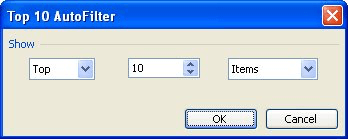
Figure 1. The Top 10 AutoFilter dialog box.

4. Adjust the center control from 10 to 5.
5. Click on OK. Excel displays the top five salaries in the list.

When you follow these steps, you may actually end up with more than five records visible, particularly if there are ties in the employee salaries. The filter identifies the top five salaries and then displays all the records with salaries matching those.

If you don't want to use the AutoFilter, another option is to simply make sure that there is something unique about each of the records in your employee list. For instance, if the employee names are in column B and the salaries are in column C, then you could use the following formula in column A to make each record unique:

=C2+ROW()/100000000

This will add the row number divided by 100,000,000 and will make a unique value. If you have (for example) identical salaries of 98,765.43 in rows 2 and 49 in column A they will be:

98765.43000002
98765.43000049

The large number (100,000,000) is so that if you had an identical number in row 65536, you would get:

98765.43065536

And even in this case the rounded value to 2 decimal places would still be the real number. If the LARGE and VLOOKUP are done with the "non-unique" values in column A, then you will return the largest salaries (and their associated people), based on the person's position within the list.

A third approach is to use the RANK and COUNTIF functions to return a unique "ranking" for each value in the list of salaries. If the salaries are in the range B1:B50, enter the following in cell C1 and copy it down the range:

=RANK(B1,$B$1:$B$50)+COUNTIF($B$1:B1,B1)-1

You can now use INDEX on the ranking values to return the name associated with each salary.

Finally, a fourth approach is to create a macro that can return the desired information. There are many ways that a macro could be implemented; the following is just one of them:

Function VLIndex(vValue, rngAll As Range, _
  iCol As Integer, lIndex As Long)
    Dim x As Long
    Dim lCount As Long
    Dim vArray() As Variant
    Dim rng As Range
    On Error GoTo errhandler

    Set rng = Intersect(rngAll, rngAll.Columns(1))
    ReDim vArray(1 To rng.Rows.Count)
    lCount = 0
    For x = 1 To rng.Rows.Count
        If rng.Cells(x).Value = vValue Then
            lCount = lCount + 1
            vArray(lCount) = rng.Cells(x).Offset(0, iCol).Value
        End If
    Next x

    ReDim Preserve vArray(1 To lCount)
    If lCount = 0 Then
        VLIndex = CVErr(xlErrNA)
    ElseIf lIndex > lCount Then
        VLIndex = CVErr(xlErrNum)
    Else
        VLIndex = vArray(lIndex)
    End If
errhandler:
    If Err.Number <> 0 Then VLIndex = CVErr(xlErrValue)
End Function

The parameters passed to this user-defined function are the value, the range of cells to lookup in, the "offset" from this range for the lookup (the number of columns to the right is positive, to the left is negative) and the number of the duplicate (1 is first value, 2 the second, and so on).

To use it, for example's sake, assume A1:B1 contain column headers, A2:A100 contains the salaries, and B2:B100 contains the employee names. In cell E2 you can enter the following to determine the largest salary in the table:

=LARGE($A$2:$A$100,ROW()-1)

In cell F2 you can enter the following formula to determine if the row has any duplicates and keep track of the current "value" of that duplicate:

=IF(E2=E1,1+F1,1)

In cell G2 you can use the following formula, which invokes the user-defined function:

=VLIndex(E2,$A$2:$A$100,1,F2)

Copy cells E2:G2 to E3:G6, and you will have (in column G) the names of the employees with the five largest salaries.

ExcelTips is your source for cost-effective Microsoft Excel training. This tip (3077) applies to Microsoft Excel 97, 2000, 2002, and 2003.