Defeating Automatic Date Parsing

Excel is normally pretty smart when it comes to importing data, but sometimes the automatic parsing it uses can be a real bother. For instance, you may import information that contains text strings, such as "1- 4- 9" (without the quotes). This is fine, but if you do a Replace to get rid of the spaces, Excel automatically converts the resulting string (1-4-9) to a date (1/4/09).

One potential solution is to copy your information to Word and do your searching and replacing there. The problem with this solution is that when you paste the information back into Excel, it will again be parsed as date information and automatically converted to the requisite date serial numbers.

The only satisfactory solution is to make sure that Excel absolutely treats the resulting strings as just that—strings—and not as dates. This can be done in one of two ways: just make sure that the original text begins with either an apostrophe or a space. This can be ensured by using the Replace feature of Excel (depending on the data you have to work with) or by using the Replace feature of Word (which is much more versatile).

With an apostrophe or space at the beginning of the cell entry, you can remove additional spaces or characters from the cell contents. If the result is text that looks like a date, Excel will not parse it as such because the leading apostrophe or space forces treatment as text.

Another way to perform the task is to follow these steps. (Assume that the original data is in the range A2:A101).

1. Insert a column to the right of the original data.
2. In cell B2, enter the following formula:

       =SUBSTITUTE(A2," ","")

1. Copy the contents of B2 into the range B3:B101.
2. Select the cells in the range of B2:B101.
3. Press Ctrl+C to copy the range to the Clipboard.
4. Select cell A2.
5. Choose Paste Special from the Edit menu. Excel displays the Paste Special dialog box. (See Figure 1.)



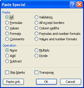
Figure 1. The Paste Special dialog box.

6. Make sure the Values option is selected.
7. Click on OK.
8. Delete column B.

These steps work because the output of the SUBSTITUTE function is always treated as text. When you copy and paste text values, they are treated as text with no additional parsing done by Excel.

ExcelTips is your source for cost-effective Microsoft Excel training. This tip (3019) applies to Microsoft Excel 97, 2000, 2002, and 2003. You can find a version of this tip for the ribbon interface of Excel (Excel 2007 and later) here: Defeating Automatic Date Parsing.