Please Note: This article is written for users of the following Microsoft Excel versions: 97, 2000, 2002, and 2003. If you are using a later version (Excel 2007 or later), this tip may not work for you. For a version of this tip written specifically for later versions of Excel, click here: Creating Two-Line Custom Formats.
Written by Allen Wyatt (last updated November 7, 2020)
This tip applies to Excel 97, 2000, 2002, and 2003
Excel is quite flexible in how it allows you to set up custom formats for displaying all sorts of values. Most custom formats are straightforward and easy to figure out, once you understand how custom formats work. (Custom formats and how to set them up has been discussed fully in other issues of ExcelTips.)
What if you want to create a two-line custom format, however? For instance, you may want to format a date so that the abbreviated day of the week and day of the month is on the first line, followed by the unabbreviated name of the month on the second line. Using such a format, a date would appear in a single cell in this manner:
Sat 4
March
Most of this can be done by the custom format "ddd d mmmm", but you need to figure out a way to add a line break between the "d" and the "mmmm". Excel won't let you press Alt+Enter between them, which is what you normally do to add a line break.
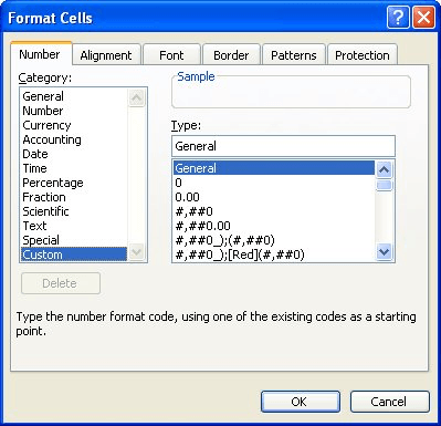
The solution is to use the numeric keypad to enter the desired line break in the format. Follow these steps to set it up:

Figure 1. The Number tab of the Format Cells dialog box.

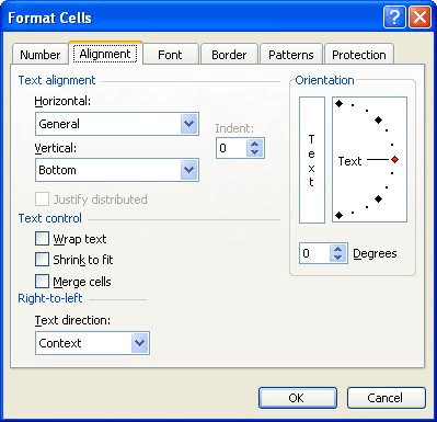
Figure 2. The Alignment tab of the Format Cells dialog box.
After setting up the format in this manner, you will need to adjust the row height of the formatted cells so that the entire two lines of the date will display.
ExcelTips is your source for cost-effective Microsoft Excel training. This tip (2895) applies to Microsoft Excel 97, 2000, 2002, and 2003. You can find a version of this tip for the ribbon interface of Excel (Excel 2007 and later) here: Creating Two-Line Custom Formats.

Program Successfully in Excel! This guide will provide you with all the information you need to automate any task in Excel and save time and effort. Learn how to extend Excel's functionality with VBA to create solutions not possible with the standard features. Includes latest information for Excel 2024 and Microsoft 365. Check out Mastering Excel VBA Programming today!
Is the information in your cells too jammed up? Here are some ways you can add some white space around that information ...
Discover MoreYou can shade your cells by filling them with a pattern. Here's how to select the pattern you want used.
Discover MoreExcel allows you to adjust not only the horizontal alignment of values in a cell, but also the vertical alignment. This ...
Discover MoreFREE SERVICE: Get tips like this every week in ExcelTips, a free productivity newsletter. Enter your address and click "Subscribe."
2025-08-08 16:42:15
Bob
Tried this in excel 2007 and it doesn't work on dates. I just get a bunch of hashes if I change the cell width, no matter how high I make the cell.
2022-11-13 06:58:43
Alex Blakenburg
To overcome the with the width issue that is frequently mentioned. The below worked for me on MS 365.
• Go into Format Cells > Alignment
• Turn Wrap text off (uncheck), if it is already checked
• Turn on Shrink to fit
• Turn Wrap text on
You should now be able to shrink the column to suit the text without it turning into ####
2022-06-02 03:40:25
Luke
Many thanks - that worked (almost) perfectly. I noticed that when I adjust the column width Excel doesn't recognize the line break and assumes the full character width (regardless of the line break). If I narrow the width I get the formatting showing as "**************".
Thanks once again
2020-12-01 12:11:04
Joe
Thanks for the tip. Problem is that column width can not be set to less than full length format, display becomes ####... negating the value of multi-line display.
2020-11-24 04:39:41
Rick Rothstein
You discovered the downside of this custom format... Excel displays it on two lines but sees it a single line of text and calculates the required cell width based on that. The only way to minimize the effect after auto-sizing the column width is to set the cell's horizontal alignment to center align, then it won't look as bad.
2020-11-23 12:14:29
Lee Wylie
I was looking to make my date narrower as I've got a workbook with data in columns by date, and management wanted the date reformatted to fit more on screen without reducing zoom. They requested this;
ddd d
mmm yy
Which would display as
Mon 23
Nov 20
This tip works in terms of displaying the text over 2 lines, which is great - however I cannot get the text to display correctly if I narrow the column width to fit the new date format, it just displays the ###### placeholder. When I autofit the columns, it adds a huge amount of white space either side, so this formatting method won't work for me.
To overcome this I had to hide the row containing dates, and use a formula;
=TEXT(B1,"ddd d") & char(10) & TEXT(B1,"mmm yy")
It's not elegant but it works.
2020-11-07 10:07:23
Rick Rothstein
Two comments about Step 6 in your tip...
1) Instead of typing ALT+0010 you can type CTRL+J and it will work the same way.
2) On my version of Excel, what I typed does not disappear when I type either of the keystrokes in #1 above; rather, the cursor seems to disappear... actually it has moved below the displayed field (if you look carefully, you can see what looks like a single blinking dot... that is the top of the blinking cursor that is now below the bottom of the Type textbox). While you cannot see what you are typing down there, you can watch the results of your typing in the Sample textbox.
Got a version of Excel that uses the menu interface (Excel 97, Excel 2000, Excel 2002, or Excel 2003)? This site is for you! If you use a later version of Excel, visit our ExcelTips site focusing on the ribbon interface.
FREE SERVICE: Get tips like this every week in ExcelTips, a free productivity newsletter. Enter your address and click "Subscribe."
Copyright © 2026 Sharon Parq Associates, Inc.
Comments