Advanced Filtering

There are some situations in which AutoFilter just doesn't have the muscle you need when processing your data. For instance, you might need to perform a calculation in a filter comparison. In these cases, you can use the advanced filtering capabilities of Excel.

Advanced filtering requires that you set up a criteria range in your worksheet. This criteria range is not part of your data list, but instead is used to signify how you want filtering to be performed. Typically, you would place your criteria before your data list, but you can also place it after. The important thing is that you separate your criteria from you data list by at least one empty row. Otherwise, Excel may think that the criteria are part of the actual data list.

The criteria are entered in your worksheet such that each column represents a different logical AND comparison, and each row represents a different logical OR comparison. If this sounds confusing, don't be concerned. An example will help clear things up.

Let's say you have a data list that starts in the sixth row of a worksheet. You have set aside the rows above this to specify your filtering criteria. The data list contains columns that describe information in your inventory. There are columns for item numbers, description, location, quantity, value, and the like. There is also a calculated column that indicates the profit derived from each inventory item.

At some time you may want to filter your data list so it shows only a limited subset of your inventory items. For instance, you might want to see only those items for which the quantity is over 2500 and profit is less than 1000, or those items where the quantity is greater than 7500, or those items where profit is under 100. (This is much more complex than you can perform using an custom AutoFilter.)

To set up such a filter, all you need to do is set your criteria. In this case, you would use cells A1:B4 as follows:

In this example the first row shows the field names to be used in comparisons, while the second through fourth rows define the actual comparisons. Notice that because there are two tests in the second row, these are considered an AND condition, and those on the other rows are considered OR conditions.

To apply these filtering criteria, follow these steps:

1. Select any cell in the data list (not in the criteria).
2. Choose Filter from the Data menu, then choose Advanced Filter. Excel displays the Advanced Filter dialog box (See Figure 1.) with the address of your original data table already filled in, in the List Range box.



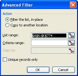
Figure 1. The Advanced Filter dialog box.

3. Select the Criteria Range field. The insertion point should appear within the field.
4. Use the mouse to select the criteria range, cells A1:B4.
5. Click on OK.