Getting Rid of Negative Zero Amounts

When you are creating a worksheet, and you format your cells to display information just the way you want, you may notice that you end up with "negative zero" amounts. Everyone learned in math classes that zero is not a negative number. So why does Excel show some zero amounts as negative?

The reason is because your formatting may call for displaying less information than Excel uses internally for its calculations. For instance, Excel keeps track of numbers out to fifteen decimal places. If your display only shows two decimal places, it is possible that a calculated value could be very small, and when rounded show as zero. If the calculated value is something like –0.000001325, then the value would show with only two digits to the right of the decimal point as –0.00. The negative sign shows, of course, because the internal value maintained by Excel is below zero.

There are a couple of ways you can solve this problem. The first is to simply round the calculated value to the desired number of decimal places. For instance, assume that this is your normal formula—the one that results in the "negative zero" values:

=SUM(A3:A23)

You can round the value in the cell by simply using the following formula instead:

=ROUND(SUM(A3:A23),2)

This usage results in the value being rounded to two decimal places. In this way you should never end up with another "negative zero" value.

Another solution preferred by some people is to force Excel to use the same internal precision as what you have displayed in your worksheet. Just follow these steps:

1. Choose Options from the Tools menu. Excel displays the Options dialog box.
2. Make sure the Calculation tab is selected. (See Figure 1.)



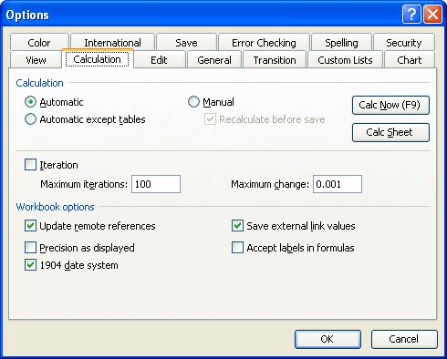
Figure 1. The Calculation tab of the Options dialog box.

3. Ensure that the Precision As Displayed check box is selected.
4. Click on OK.

ExcelTips is your source for cost-effective Microsoft Excel training. This tip (2576) applies to Microsoft Excel 97, 2000, 2002, and 2003. You can find a version of this tip for the ribbon interface of Excel (Excel 2007 and later) here: Getting Rid of Negative Zero Amounts.