Please Note: This article is written for users of the following Microsoft Excel versions: 97, 2000, 2002, and 2003. If you are using a later version (Excel 2007 or later), this tip may not work for you. For a version of this tip written specifically for later versions of Excel, click here: Conditional Formatting with Data Imported from Access.
Written by Allen Wyatt (last updated October 1, 2022)
This tip applies to Excel 97, 2000, 2002, and 2003
Cory is having a problem getting his conditional formatting to work as desired with information imported into Excel from Access. The data being imported in a particular column can either be text (such as "17 U") or numeric (such as 32). The conditional format checks to see if the value in the cell is greater than zero, in which case the value is underlined. This won't work properly with the imported data because not only does Excel treat the text (17 U) as text, but it also treats the numeric (32) as text. This makes sense, since Excel treats the entire column as text rather than changing data format for each cell in the column.
There are a couple of ways you can fix this problem. One is to change the formula you are using in your conditional format. Instead of checking to see if the value is greater than zero, use the following formula (set the conditional check to "Format Is"):
=VALUE(E3) > 0
This formula uses the VALUE function to check what is in cell E3. If the contents are a number—even if it is formatted as text by Excel—then the formula returns True and the condition is met for the formatting. If the contents of E3 really are text (as in "17 U"), then the formula returns a #VALUE error, which does not satisfy the condition and the formatting is not applied.
Another approach is to force Excel to evaluate the imported cells and convert them to numeric values, if appropriate. An easy way to do this is as follows:
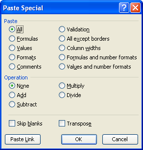
Figure 1. The Paste Special dialog box.
What you just did was to "add" the contents of the Clipboard to all the cells you selected in step 3. If the cells contained real text, then nothing happened to those cells; they remain the same and are still treated as text. If the cells contained a numeric value, then Excel treats it as a number and adds zero to it. This value, as a numeric, is deposited back in the cell, and treated as a real number. This means that the conditional formatting test that you previously set up should work just fine on those cells since they are no longer treated as text.
ExcelTips is your source for cost-effective Microsoft Excel training. This tip (2418) applies to Microsoft Excel 97, 2000, 2002, and 2003. You can find a version of this tip for the ribbon interface of Excel (Excel 2007 and later) here: Conditional Formatting with Data Imported from Access.

Create Custom Apps with VBA! Discover how to extend the capabilities of Office 365 applications with VBA programming. Written in clear terms and understandable language, the book includes systematic tutorials and contains both intermediate and advanced content for experienced VB developers. Designed to be comprehensive, the book addresses not just one Office application, but the entire Office suite. Check out Mastering VBA for Microsoft Office 365 today!
You can use conditional formatting to add shading to various cells in your worksheet. This tip shows how you can shade ...
Discover MoreConditional formatting is very powerful, but at some point you may want to make the formatting "unconditional." In other ...
Discover MoreNeed to have a sound played if a certain condition is met? It is rather easy to do if you use a user-defined function to ...
Discover MoreFREE SERVICE: Get tips like this every week in ExcelTips, a free productivity newsletter. Enter your address and click "Subscribe."
There are currently no comments for this tip. (Be the first to leave your comment—just use the simple form above!)
Got a version of Excel that uses the menu interface (Excel 97, Excel 2000, Excel 2002, or Excel 2003)? This site is for you! If you use a later version of Excel, visit our ExcelTips site focusing on the ribbon interface.
FREE SERVICE: Get tips like this every week in ExcelTips, a free productivity newsletter. Enter your address and click "Subscribe."
Copyright © 2025 Sharon Parq Associates, Inc.
 Please Note:
This article is written for users of the following Microsoft Excel versions: 97, 2000, 2002, and 2003. If you are using a later version (Excel 2007 or later), this tip may not work for you. For a version of this tip written specifically for later versions of Excel, click here:
Please Note:
This article is written for users of the following Microsoft Excel versions: 97, 2000, 2002, and 2003. If you are using a later version (Excel 2007 or later), this tip may not work for you. For a version of this tip written specifically for later versions of Excel, click here:
Comments