Checking for Duplicate Rows Based on a Range of Columns

Jennifer has a lot of data in a worksheet, and she considers some of the rows to be duplicates. She determines whether a row is a duplicate based upon whether a range of columns in one row is identical to the same range of columns in the previous row. For instance, if all of the values in F7:AB7 are identical to the values in F6:AB6, the Jennifer would consider row 7 to be a duplicate of row 6. She wonders if there is a way that she can easily check for such duplicate rows and highlight the duplicates in some manner.

One approach to this problem is to utilize the conditional formatting capabilities of Excel. If your data is in rows A1:AZ100, then select the range You could then use the following as a formulaic test within your conditional format:

=IF(AND($F2:$AB2=$F1:$AB1),1,0)=1

If your conditional format applies a color to the cells, then you'll see the color appear anytime the values in columns F through AB are equal to the values in the same columns of the row directly above the one that is colored.

If Jennifer's data consists only of cells in the columns F:AB, then she can use the filtering capabilities of Excel to mark the duplicate rows. Here are the general steps:

1. Select the cells containing your data. For instance, if the first row contains column headers, you should select F2:AB100.
2. Apply a color to those cells, so that all the data is shaded some unique color.
3. Select any cell in data table.
4. Choose Filter from the Data menu, then choose Advanced Filter from the resulting submenu. Excel displays the Advanced Filter dialog box. (See Figure 1.)



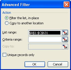
Figure 1. The Advanced Filter dialog box.

5. Make sure that Filter the List, In Place is selected. (It should be selected by default.)
6. Click the Unique Records Only check box.
7. Click OK. Excel collapses your data so that only unique (non-duplicate) records are shown.
8. Select the visible rows of data.
9. Remove the color you applied in step 2.
10. Remove the filter you applied in steps 4 through 7.

At this point, only the duplicate records are highlighted with the color you used in step 2. These records can be safely deleted, leaving only the unique records.

ExcelTips is your source for cost-effective Microsoft Excel training. This tip (10607) applies to Microsoft Excel 97, 2000, 2002, and 2003. You can find a version of this tip for the ribbon interface of Excel (Excel 2007 and later) here: Checking for Duplicate Rows Based on a Range of Columns.