Please Note: This article is written for users of the following Microsoft Excel versions: 97, 2000, 2002, and 2003. If you are using a later version (Excel 2007 or later), this tip may not work for you. For a version of this tip written specifically for later versions of Excel, click here: Tying a Hyperlink to a Specific Cell.
Manoj created a hyperlink between two worksheets by using copy and paste hyperlink command (the hyperlink targets a specific cell). Later he inserted some rows on the target worksheet that caused the target cell to move down a bit. Even though the target cell moves down, the hyperlink continues to reference the old cell location. Manoj is wondering if there is a way to make sure that the hyperlink always targets the cell he intended when creating the link.
In Excel, hyperlink addresses are essentially text that references a cell. Formulas in Excel link to cell references which adjust when changes in the worksheet structure are made (inserting and deleting rows and columns, etc.). Hyperlink addresses, being text instead of cell references, will not adjust with such changes.
The solution is to create a named range that refers to the target cell you want used in the hyperlink. (You do this by choosing Insert | Name | Define.) When you create your hyperlink, you can then reference this named range in the Insert Hyperlink dialog box. (See Figure 1.)
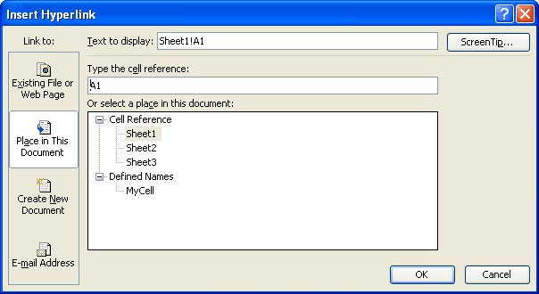
Figure 1. The Insert Hyperlink dialog box.
At the left of the dialog box, click Place In This Document. You'll then see a list of named ranges in your workbook and you can choose which one you want to be associated with this hyperlink. In this way, you allow Excel to take care of translating between the name and the address for that name, which means that the hyperlink will always point to the cell you want it to point to.
ExcelTips is your source for cost-effective Microsoft Excel training. This tip (3466) applies to Microsoft Excel 97, 2000, 2002, and 2003. You can find a version of this tip for the ribbon interface of Excel (Excel 2007 and later) here: Tying a Hyperlink to a Specific Cell.

Best-Selling VBA Tutorial for Beginners Take your Excel knowledge to the next level. With a little background in VBA programming, you can go well beyond basic spreadsheets and functions. Use macros to reduce errors, save time, and integrate with other Microsoft applications. Fully updated for the latest version of Office 365. Check out Microsoft 365 Excel VBA Programming For Dummies today!
Hyperlinks can be helpful in some worksheets but bothersome in others. Here's how to get rid of any hyperlinks you don't ...
Discover MoreNeed a quick link within a document to some external data? You can paste information so that Excel treats it just like a ...
Discover MoreMany people like to use Excel to keep track of lists of hyperlinks. Want to keep a permanent record of which hyperlinks ...
Discover MoreFREE SERVICE: Get tips like this every week in ExcelTips, a free productivity newsletter. Enter your address and click "Subscribe."
There are currently no comments for this tip. (Be the first to leave your comment—just use the simple form above!)
Got a version of Excel that uses the menu interface (Excel 97, Excel 2000, Excel 2002, or Excel 2003)? This site is for you! If you use a later version of Excel, visit our ExcelTips site focusing on the ribbon interface.
FREE SERVICE: Get tips like this every week in ExcelTips, a free productivity newsletter. Enter your address and click "Subscribe."
Copyright © 2026 Sharon Parq Associates, Inc.
 Please Note:
This article is written for users of the following Microsoft Excel versions: 97, 2000, 2002, and 2003. If you are using a later version (Excel 2007 or later), this tip may not work for you. For a version of this tip written specifically for later versions of Excel, click here:
Please Note:
This article is written for users of the following Microsoft Excel versions: 97, 2000, 2002, and 2003. If you are using a later version (Excel 2007 or later), this tip may not work for you. For a version of this tip written specifically for later versions of Excel, click here:
Comments