Please Note: This article is written for users of the following Microsoft Excel versions: 97, 2000, 2002, and 2003. If you are using a later version (Excel 2007 or later), this tip may not work for you. For a version of this tip written specifically for later versions of Excel, click here: Matching Formatting when Concatenating.
Written by Allen Wyatt (last updated October 1, 2022)
This tip applies to Excel 97, 2000, 2002, and 2003
When using a formula to merge the contents of multiple cells into one cell, Kris is having trouble getting Excel to preserve the formatting of the original cells. For example, assume that cells A1 and B1 contain 1 and 0.33, respectively. In cell C1, he enters the following formula:
=A1 & " : " & B1
The result in cell C1 looks like this:
1 : 0.3333333333
The reason that the resulting C1 doesn't match what is shown in B1 (0.33) is because the value in B1 isn't really 0.33. Internally, Excel maintains values to 15 digits, so that if cell B1 contains a formula such as =1/3, internally this is maintained as 0.33333333333333. What you see in cell B1, however, depends on how the cell is formatted. In this case, the formatting probably is set to display only two digits beyond the decimal point.
There are several ways you can get the desired results in cell C1, however. One method is to simply modify your formula a bit so that the values pulled from cells A1 and B1 are formatted. For instance, the following example uses the TEXT function to do the formatting:
=TEXT(A1,"0") & " : " & TEXT(B1,"0.00")
In this case, A1 is formatted to display only whole numbers and B1 is formatted to display only two decimal places.. You could also use the ROUND function to achieve a similar result:
=ROUND(A1,0) & " : " & ROUND(B1,2)
Another possible solution is to change how Excel deals with precision in the workbook. Follow these steps:
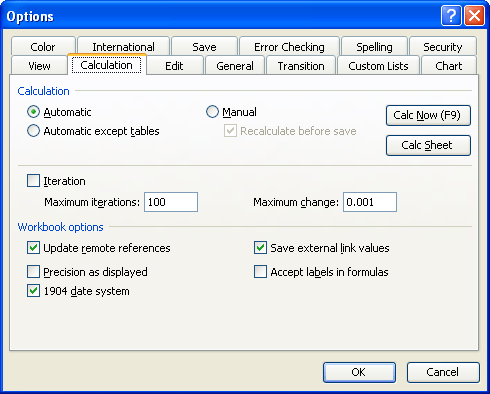
Figure 1. The Calculation tab of the Options dialog box.
Now, Excel uses the precision shown on the screen in all of its calculations and concatenations instead of doing calculations at the full 15-digit precision it normally maintains. While this approach may be acceptable for some users, for others it will present more problems than it solves. You will need to determine if you can live with the lower precision in order to get the output formatted the way you expect.
Still another approach is to create your own user-defined function that will return what is displayed for the target cell, rather than what is stored there. The following macro will work great in this regard:
Function FmtText(rng As Range)
    Application.Volatile
    FmtText = rng.Cells(1).Text
End Function
To use this macro, you would use a formula like this in your worksheet:
=FmtText(A1) & " : " & FmtText(B1)
Note:
ExcelTips is your source for cost-effective Microsoft Excel training. This tip (3213) applies to Microsoft Excel 97, 2000, 2002, and 2003. You can find a version of this tip for the ribbon interface of Excel (Excel 2007 and later) here: Matching Formatting when Concatenating.

Solve Real Business Problems Master business modeling and analysis techniques with Excel and transform data into bottom-line results. This hands-on, scenario-focused guide shows you how to use the latest Excel tools to integrate data from multiple tables. Check out Microsoft Excel Data Analysis and Business Modeling today!
Insert or delete a column, and Excel automatically updates references within formulas that are affected by the change. If ...
Discover MoreSearching for a value using Excel's Find tool is easy; searching for that same value using a formula or a macro is more ...
Discover MoreDo you see some small rectangular boxes appearing in your formula results? It could be because Excel is substituting that ...
Discover MoreFREE SERVICE: Get tips like this every week in ExcelTips, a free productivity newsletter. Enter your address and click "Subscribe."
There are currently no comments for this tip. (Be the first to leave your comment—just use the simple form above!)
Got a version of Excel that uses the menu interface (Excel 97, Excel 2000, Excel 2002, or Excel 2003)? This site is for you! If you use a later version of Excel, visit our ExcelTips site focusing on the ribbon interface.
FREE SERVICE: Get tips like this every week in ExcelTips, a free productivity newsletter. Enter your address and click "Subscribe."
Copyright © 2026 Sharon Parq Associates, Inc.
 Please Note:
This article is written for users of the following Microsoft Excel versions: 97, 2000, 2002, and 2003. If you are using a later version (Excel 2007 or later), this tip may not work for you. For a version of this tip written specifically for later versions of Excel, click here:
Please Note:
This article is written for users of the following Microsoft Excel versions: 97, 2000, 2002, and 2003. If you are using a later version (Excel 2007 or later), this tip may not work for you. For a version of this tip written specifically for later versions of Excel, click here:
Comments