Conditional Formats that Distinguish Blanks and Zeroes

Let's say that you routinely import information from another program into Excel. The information contains numeric values, but it can also contain blanks. You might want to use a conditional format on the imported information to highlight any zero values. The problem is, if you just add a conditional format that highlights the cells to see if they are zero, then the condition will also highlight any cells that are blank, since they contain a "zero" value, as well.

There are several different solutions to this predicament. One solution is to apply a conditional format that uses two conditions. The first condition checks for the blanks, and the second checks for zero values. The condition that checks for blanks doesn't need to adjust any formatting, but the one that checks for zero values can. This works because if the first condition is satisfied (the cell is blank), the second condition is never tested. Do the following:

1. Select the range you want conditionally formatted. (For this example, I'll assume that you've selected the range A2:A99.)
2. Choose Conditional Formatting from the Format menu. Excel displays the Conditional Formatting dialog box.
3. Using the first drop-down list for Condition 1, choose Formula Is.
4. In the formula box for Condition 1, enter the formula =ISBLANK(A2). (See Figure 1.)



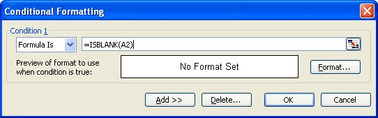
Figure 1. The Conditional Formatting dialog box after setting one condition.

5. Click Add. Excel adds a second condition to the dialog box.
6. Using the first drop-down list for Condition 2, choose Cell Value Is.
7. Using the second drop-down list for Condition 2, choose Equal To
8. In the value box for Condition 2, enter 0. (See Figure 2.)



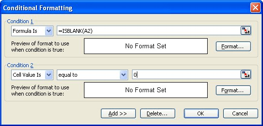
Figure 2. The Conditional Formatting dialog box after setting two conditions.

9. Click the Format button for Condition 2. Excel displays the Format Cells dialog box.
10. Use the controls in the dialog box to modify the formatting, as desired.
11. Click OK to close the Format Cells dialog box.
12. Click OK to close the Conditional Formatting dialog box. The formatting is applied to the range of cells you selected in step 1.

Another solution is to combine your two conditions into a single condition. Follow these steps:

1. Select the range you want conditionally formatted. (For this example, I'll assume that you've selected the range A2:A99.)
2. Choose Conditional Formatting from the Format menu. Excel displays the Conditional Formatting dialog box.
3. Using the first drop-down list for Condition 1, choose Formula Is.
4. In the formula box for Condition 1, enter the formula =AND(A2=0,A2<>"").
5. Click the Format button for Condition 1. Excel displays the Format Cells dialog box.
6. Use the controls in the dialog box to modify the formatting, as desired.
7. Click OK to close the Format Cells dialog box.
8. Click OK to close the Conditional Formatting dialog box. The formatting is applied to the range of cells you selected in step 1.

The formula used in step 4 checks to make sure that the value is 0 and that the cell is not blank. The AND function makes sure that only when both criteria are satisfied will the formula return True and the format be applied.

There are any number of other formulas that could also be used. For instance, each of the following formulas could be substituted in either step 5 or 4:

• =AND(COUNT(A2)=1,A2=0)
• =AND(A2=0,NOT(ISBLANK(A2)))
• =AND(A2=0,LEN(A2)>0)
• =NOT(ISBLANK(A2))*(A2=0)

If you wanted an even faster way to highlight zero values while ignoring blanks, you might consider using a macro. The macro would be faster because you could just import and run it; you don't have to select a range of cells and enter the formula (or formulas) for the conditional formatting. The following macro is an example of one you could use:

Sub FormatRed()
    TotalRows = 65000
    ColNum = 1

    For i = 1 To Cells(TotalRows, ColNum).End(xlUp).Row
        Cells(i, ColNum).Interior.ColorIndex = xlAutomatic
        If IsNumeric(Cells(i, ColNum).Value) Then
            If Cells(i, ColNum).Value = 0 Then
                Cells(i, ColNum).Interior.ColorIndex = 3
            End If
        End If
    Next
End Sub

The macro checks the cells in column A. (It checks the cells in rows 1 through 65,000; you can modify this, if desired.) If the cell contains a numeric value and that value is zero, then the cell is filled with red. If the cell contains something else, then the cell is set back to its normal color.

ExcelTips is your source for cost-effective Microsoft Excel training. This tip (2980) applies to Microsoft Excel 97, 2000, 2002, and 2003. You can find a version of this tip for the ribbon interface of Excel (Excel 2007 and later) here: Conditional Formats that Distinguish Blanks and Zeroes.