Please Note: This article is written for users of the following Microsoft Excel versions: 97, 2000, 2002, and 2003. If you are using a later version (Excel 2007 or later), this tip may not work for you. For a version of this tip written specifically for later versions of Excel, click here: Shading Rows with Conditional Formatting.
If you haven't tried out the conditional formatting features of Excel before, they can be quite handy. One way to use this feature is to cause Excel to shade every other row in a table. This is great when you have a particularly wide table, and you want to make it a bit easier to read on printouts. Simply follow these steps:
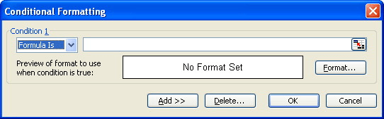
Figure 1. The Conditional Formatting dialog box.
=MOD(ROW(),2)=0
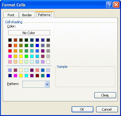
Figure 2. The Patterns tab of the Format Cells dialog box.
Note:
ExcelTips is your source for cost-effective Microsoft Excel training. This tip (2799) applies to Microsoft Excel 97, 2000, 2002, and 2003. You can find a version of this tip for the ribbon interface of Excel (Excel 2007 and later) here: Shading Rows with Conditional Formatting.

Excel Smarts for Beginners! Featuring the friendly and trusted For Dummies style, this popular guide shows beginners how to get up and running with Excel while also helping more experienced users get comfortable with the newest features. Check out Excel 2019 For Dummies today!
Conditional formatting is a great tool. You may need to use this tool to tell the difference between cells that are empty ...
Discover MoreConditional formatting can be a great way to highlight specific information in your worksheets. This tip explains the ...
Discover MoreThere are many times when you are creating a worksheet that you need to analyze dates within that worksheet. Once such ...
Discover MoreFREE SERVICE: Get tips like this every week in ExcelTips, a free productivity newsletter. Enter your address and click "Subscribe."
There are currently no comments for this tip. (Be the first to leave your comment—just use the simple form above!)
Got a version of Excel that uses the menu interface (Excel 97, Excel 2000, Excel 2002, or Excel 2003)? This site is for you! If you use a later version of Excel, visit our ExcelTips site focusing on the ribbon interface.
FREE SERVICE: Get tips like this every week in ExcelTips, a free productivity newsletter. Enter your address and click "Subscribe."
Copyright © 2026 Sharon Parq Associates, Inc.
 Please Note:
This article is written for users of the following Microsoft Excel versions: 97, 2000, 2002, and 2003. If you are using a later version (Excel 2007 or later), this tip may not work for you. For a version of this tip written specifically for later versions of Excel, click here:
Please Note:
This article is written for users of the following Microsoft Excel versions: 97, 2000, 2002, and 2003. If you are using a later version (Excel 2007 or later), this tip may not work for you. For a version of this tip written specifically for later versions of Excel, click here:
Comments