Please Note: This article is written for users of the following Microsoft Excel versions: 97, 2000, 2002, and 2003. If you are using a later version (Excel 2007 or later), this tip may not work for you. For a version of this tip written specifically for later versions of Excel, click here: Using Fractional Number Formats.
Excel supports fractional number formats when displaying numbers in a cell. In some industries, fractions are the norm. For instance, the building industry routinely uses fractions to measure lumber and distances. If you format a cell correctly, you can enter a number as 12.25 and have it displayed as 12 1/4.
You can specify a pre-defined fractional number format by following these steps:
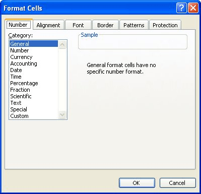
Figure 1. The Number tab of the Format Cell dialog box.
Even though you can use the predefined fractional formats, there is a good chance these will not meet all your fractional needs. When you define your own fraction formats, Excel assumes that if you provide digit place holders on both sides of the slash (/), you are defining a fractional format. For instance, if you are working with inches, you can define the following format:
#-#/##\"
This results in numbers such as 18.75 being displayed as 18-3/4". (The backslash indicates that the following character should be used literally as is, in this case the quote mark.) This is exactly what the building contractor may need to convey specifications or other measurements.
When you define fractional formats, make sure you use, as the denominator to the fraction, the maximum number of digits you want to appear there. Since there are two digits in the denominator of the above example, the largest fraction that can be displayed using this format is 98/99. If you want larger denominators, you must format for them explicitly, as in:
#–#/###\"
ExcelTips is your source for cost-effective Microsoft Excel training. This tip (2759) applies to Microsoft Excel 97, 2000, 2002, and 2003. You can find a version of this tip for the ribbon interface of Excel (Excel 2007 and later) here: Using Fractional Number Formats.

Create Custom Apps with VBA! Discover how to extend the capabilities of Office 365 applications with VBA programming. Written in clear terms and understandable language, the book includes systematic tutorials and contains both intermediate and advanced content for experienced VB developers. Designed to be comprehensive, the book addresses not just one Office application, but the entire Office suite. Check out Mastering VBA for Microsoft Office 365 today!
You may want Excel to format your dates using a pattern it doesn't normally use—such as using periods instead of ...
Discover MoreThe error message "too many cell formats" can be difficult to fix. This tip describes ways you can attempt to get rid of ...
Discover MoreThere are times when displaying zero values in a worksheet (especially if there are lots of them) can be distracting from ...
Discover MoreFREE SERVICE: Get tips like this every week in ExcelTips, a free productivity newsletter. Enter your address and click "Subscribe."
There are currently no comments for this tip. (Be the first to leave your comment—just use the simple form above!)
Got a version of Excel that uses the menu interface (Excel 97, Excel 2000, Excel 2002, or Excel 2003)? This site is for you! If you use a later version of Excel, visit our ExcelTips site focusing on the ribbon interface.
FREE SERVICE: Get tips like this every week in ExcelTips, a free productivity newsletter. Enter your address and click "Subscribe."
Copyright © 2026 Sharon Parq Associates, Inc.
 Please Note:
This article is written for users of the following Microsoft Excel versions: 97, 2000, 2002, and 2003. If you are using a later version (Excel 2007 or later), this tip may not work for you. For a version of this tip written specifically for later versions of Excel, click here:
Please Note:
This article is written for users of the following Microsoft Excel versions: 97, 2000, 2002, and 2003. If you are using a later version (Excel 2007 or later), this tip may not work for you. For a version of this tip written specifically for later versions of Excel, click here:
Comments