Transposing and Linking

Excel offers many different ways to paste information that you have copied. You can see these different methods when you choose the Paste Special option from the Edit menu. Two of the most popular pasting methods are transposing and linking.

• Transpose. This turns the orientation of your copied data ninety degrees. If you had previously copied five cells from a column, they are pasted as five cells in a row.
• Linking. You do this by choosing Paste Link from the Paste Special dialog box. It causes Excel to paste references to the original data instead of copied values. When you change the original data, the information is automatically changed in the place where you did the Paste Link.

Unfortunately, it seems that these two options are mutually exclusive. If you select the Transpose option, the Paste Link button is grayed out so you can no longer select it.

There are two ways you can get around this. One involves modifying the pasting process, and the other involves the use of a formula. The first method is as follows:

1. Copy the data you want to transpose and link, as you normally would.
2. Select any cell in an unused worksheet.
3. Choose Paste Special from the Edit menu. This displays the Paste Special dialog box. (See Figure 1.)



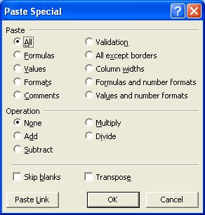
Figure 1. The Paste Special dialog box.

4. Click on the Paste Link button. Your information is pasted, as a link, in the worksheet. Make sure it remains selected.
5. Press Ctrl+H to display the Replace dialog box. (See Figure 2.)



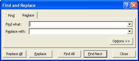
Figure 2. The Replace dialog box.

6. In the Find What area, type an equal sign.
7. In the Replace With area, type a pound sign followed by an equal sign.
8. Click on Replace All. All the information you just pasted is essentially converted from formulas into text. Make sure it remains selected.
9. Press Ctrl+C to copy the range to the Clipboard.
10. Select the cell where you want the final transposed and linked range to reside.
11. Choose Paste Special from the Edit menu. This displays the Paste Special dialog box.
12. Choose the Transpose check box.
13. Click on OK. The information is pasted, but it is transposed into the final location. Make sure it remains selected.
14. Press Ctrl+H to display the Replace dialog box.
15. In the Find What area, type a pound sign followed by an equal sign.
16. In the Replace With area, type an equal sign.
17. Click on Replace All. All the information you just pasted is converted back to formulas.

This may seem like a lot of steps, but it is not that bad in reality. Also, if you find yourself doing this procedure a lot, you can create a macro that does it for you.

If you would rather use the formula process, follow these steps:

1. Make sure the range of cells you want to link and transpose have been given a name. For this example, let's say you named it MyRange.
2. Count the number of rows and columns in the range.
3. Starting at the cell where you want the information to end up, select a range that has the opposite number of rows and columns. Thus, if the original range had 3 columns and 2 rows, the target range would have 2 columns and 3 rows.
4. Type this formula: =TRANSPOSE([Book1]Sheet1!MyRange). You should substitute different workbook, sheet, and range names, as necessary.
5. Press Shift+Ctrl+Enter.

At this point your information, linked from the original, appears in the selected range.

ExcelTips is your source for cost-effective Microsoft Excel training. This tip (2652) applies to Microsoft Excel 97, 2000, 2002, and 2003. You can find a version of this tip for the ribbon interface of Excel (Excel 2007 and later) here: Transposing and Linking.