Please Note: This article is written for users of the following Microsoft Excel versions: 97, 2000, 2002, and 2003. If you are using a later version (Excel 2007 or later), this tip may not work for you. For a version of this tip written specifically for later versions of Excel, click here: Displaying a Hidden First Column.
Excel makes it easy to hide and unhide columns. What isn't so easy is displaying a hidden column if that column is the left-most column in the worksheet. For instance, if you hide column A, Excel will dutifully follow out your instructions. If you later want to unhide column A, the solution isn't so obvious.
To unhide the left-most columns of a worksheet when they are hidden, follow these steps:
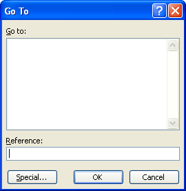
Figure 1. The Go To dialog box.
Another way to display the first column is to click on the header for column B, and then drag the mouse to the left. If you release the mouse button when the pointer is over the gray block that marks the intersection of the row and column headers (the blank gray block just above the row headers), then column B and everything to its left, including the hidden column A, are selected. You can then choose Column from the Format menu and then choose Unhide.
A third method is even niftier, provided you have a good eye and a steady mouse pointer. If you move your mouse pointer into the column header area, and then slowly move it to the left, you notice that it turns into a double-headed arrow with a blank spot in the middle as you position the pointer over the small area immediately to the left of the column B header. This double-headed arrow is a bit difficult to describe; it looks most closely like the double-headed arrow that appears when you position the pointer over the dividing line between column headers. It is different, however, because instead of a black line dividing the double arrows, there are two black lines with a gap between them.
When your mouse pointer changes to this special double-headed arrow, all you have to do is right-click and choose Unhide. Your previously missing column A magically reappears.
ExcelTips is your source for cost-effective Microsoft Excel training. This tip (2626) applies to Microsoft Excel 97, 2000, 2002, and 2003. You can find a version of this tip for the ribbon interface of Excel (Excel 2007 and later) here: Displaying a Hidden First Column.

Best-Selling VBA Tutorial for Beginners Take your Excel knowledge to the next level. With a little background in VBA programming, you can go well beyond basic spreadsheets and functions. Use macros to reduce errors, save time, and integrate with other Microsoft applications. Fully updated for the latest version of Office 365. Check out Microsoft 365 Excel VBA Programming For Dummies today!
If you get an error when you try to use one of your custom views, it could be due to the protection you have applied to ...
Discover MoreFREE SERVICE: Get tips like this every week in ExcelTips, a free productivity newsletter. Enter your address and click "Subscribe."
2023-03-23 13:05:33
Catherine Buggy
Method 2 worked perfectly. Thanks so much.
Got a version of Excel that uses the menu interface (Excel 97, Excel 2000, Excel 2002, or Excel 2003)? This site is for you! If you use a later version of Excel, visit our ExcelTips site focusing on the ribbon interface.
FREE SERVICE: Get tips like this every week in ExcelTips, a free productivity newsletter. Enter your address and click "Subscribe."
Copyright © 2026 Sharon Parq Associates, Inc.
 Please Note:
This article is written for users of the following Microsoft Excel versions: 97, 2000, 2002, and 2003. If you are using a later version (Excel 2007 or later), this tip may not work for you. For a version of this tip written specifically for later versions of Excel, click here:
Please Note:
This article is written for users of the following Microsoft Excel versions: 97, 2000, 2002, and 2003. If you are using a later version (Excel 2007 or later), this tip may not work for you. For a version of this tip written specifically for later versions of Excel, click here:
Comments