Highlighting Values in a Cell

Trev has a table of sales forecasts by product that several users review and update. The forecasts are initially set with various formulas, but the users are allowed to override the formulas by entering a value into any cell that contains one of the formulas. If a user does this, it would be helpful for Trev to have Excel somehow highlight that cell.

There are a couple of approaches you can take. First, you could use conditional formatting to do the highlighting. Set the conditional formatting to "Cell Value Is" "Not Equal To" and then enter the formula as the comparison. This will tell you when the value in the cell does not equal whatever the formula is, but a potential "gottcha" is if the person overrides the formula with the result of that formula. For instance, if the formula would have produced a result of "27" and the user types "27" into the cell.

Another possibility is to define a formula in a named constant, and then use that named constant in a conditional format. Follow these steps:

1. Choose Name from the Insert menu, then choose Define. Excel displays the Define Name dialog box. (See Figure 1.)



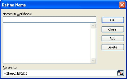
Figure 1. The Define Name dialog box.

2. In the Names in Workbook box, enter the name you want assigned to this formula. For this example, use CellHasNoFormula.
3. Select whatever is in the Refers To box, at the bottom of the dialog box, and press Del. This gets rid of whatever Excel had there before.
4. Enter the following formula in the Refers To box:

     =NOT(GET.CELL(48,INDIRECT("rc",FALSE)))

5. Click OK.

Now you can set up some conditional formats and use this named formula in the format. Simply set the condition to "Formula Is" and enter the following formula in the condition:

=CellHasNoFormula

The formula returns True or False, depending on whether there is a formula in the cell or nor. If there is no formula, then True is returned and whatever format you specify is applied to the cell.

Another approach is to use a user-defined function to return True or False, and then set up the conditional format. You could use a very simple macro, such as the following:

Function IsFormula(Check_Cell As Range) As Boolean
    Application.Volatile
    IsFormula = Check_Cell.HasFormula
End Function

You can then specify "Formula Is" in the conditional format, and use the following formula if, for instance, you are conditionally formatting cell C1:

=NOT(IsFormula(C1))

The formula returns True if there is no formula in the cell, so the conditional format is applied.

The only downside of using any of these formulas to determine if a formula is in the cell is that it cannot determine if the formula in the cell has been replaced with a different formula. This applies to both the macro approach and the defined formula approach.

A totally different approach is to rethink your worksheet a bit. You can separate cells for user input from those that use the formulas. The formula could use an IF function to see if the user entered something in the user input cell. If not, your formula would be used to determine a value; if so, then the user's input is used in preference to your formula. This approach allows you to keep the formulas you need, without them being overwritten by the user. This results in great integrity of the formulas and the worksheet results.

ExcelTips is your source for cost-effective Microsoft Excel training. This tip (3224) applies to Microsoft Excel 97, 2000, 2002, and 2003. You can find a version of this tip for the ribbon interface of Excel (Excel 2007 and later) here: Highlighting Values in a Cell.