Formatting Subtotal Rows

When you add subtotals to a worksheet, Excel automatically formats the subtotals using a bold font. You, however, may want to have some different type of formatting for the subtotals, such as shading them in yellow or a different color.

If you use subtotals sparingly and only want to apply a different format for one or two worksheets, you can follow these general steps:

1. Apply your subtotals, as desired.
2. Select the entire data table, including the subtotals.
3. Using the Outline area at the left of the screen, collapse the detail in your worksheet so that only the subtotals are showing.
4. Press F5 to display the Go To dialog box. (See Figure 1.)



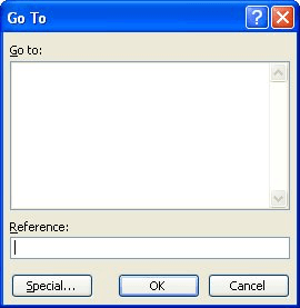
Figure 1. The Go To dialog box.

5. Click Special to display the Go To Special dialog box. (See Figure 2.)



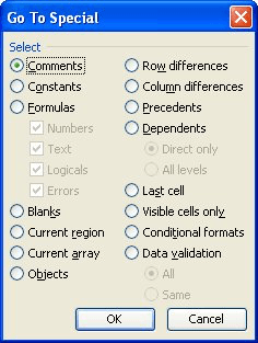
Figure 2. The Go To Special dialog box.

6. Select the Visible Cells Only option button.
7. Click OK. Now, only the visible subtotal rows are selected.
8. Apply your formatting, as desired.

If you will be repeatedly adding and removing subtotals to the same data table, you may be interested in using conditional formatting to apply the desired subtotal formatting. Follow these steps:

1. Before applying your subtotals, select your entire data table.
2. Choose Conditional Formatting from the Formatting menu. Excel displays the Conditional Formatting dialog box.
3. In the left-most drop-down list, choose Formula Is. The dialog box changes to reflect your choice. (See Figure 3.)



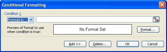
Figure 3. The Conditional Formatting dialog box.

4. In the formula box, just to the right of the drop-down list used in step 3, enter the following formula: =ISNUMBER(FIND("Grand Total",$A1))
5. Click Format to display the Format Cells dialog box.
6. Using the controls in the dialog box, set the formatting as you want it applied to the Grand Total row.
7. Click OK to dismiss the Format Cells dialog box.
8. Click Add. Excel adds a second conditional format.
9. In the left-most drop-down list of the second condition, choose Formula Is. The dialog box changes to reflect your choice.
10. In the formula box, just to the right of the drop-down list used in step 9, enter the following formula: =ISNUMBER(FIND("Total",$A1))
11. Click Format to display the Format Cells dialog box. (See Figure 4.)



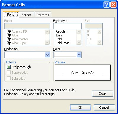
Figure 4. The Format Cells dialog box.

12. Using the controls in the dialog box, set the formatting as you want it applied to the Total row.
13. Click OK to dismiss the Format Cells dialog box.
14. Click OK to dismiss the Conditional Formatting dialog box.

When following the above steps, make sure that you replace A1 (steps 4 and 10) with the column in which your subtotals are added. Thus, if your subtotals are in column G, you would use G1 instead of A1.

If you need to do formatting of subtotals on quite a few worksheets, then you may want to create a macro that will do the formatting for you. The following macro examines all the cells in a selected range, and then applies cell coloring, as appropriate.

Sub FormatTotalRows()
    Dim rCell as Range

    For Each rCell In Selection
        If Right(rCell.Value, 5) = "Total" Then
            Rows(rCell.Row).Interior.ColorIndex = 36
        End If

        If Right(rCell.Value, 11) = "Grand Total" Then
            Rows(rCell.Row).Interior.ColorIndex = 44
        End If
    Next
End Sub

The macro colors the subtotal rows yellow and the grand total row orange. The macro, although simple in nature, is not as efficient as it could be since every cell in the selected range is inspected. Nevertheless, on a 10 column 5000 row worksheet this macro runs in under 5 seconds.

ExcelTips is your source for cost-effective Microsoft Excel training. This tip (2984) applies to Microsoft Excel 97, 2000, 2002, and 2003. You can find a version of this tip for the ribbon interface of Excel (Excel 2007 and later) here: Formatting Subtotal Rows.