Counting with Two Criteria

John has a worksheet that contains records used in a cost-tracking system. Record numbers are entered in column A, locations in column B, and costs in column C. Not all records have a cost value entered in column C. John wants to determine a count of records "with location X and cost <> 0".

Your first impulse may be to use one of the worksheet functions designed for counting, such as CountIf. The only problem is that CountIf doesn't permit two conditions to be checked in calculating a solution. There are, however, a couple of solutions you can use, without the need of adding additional columns or intermediate calculations.

The first (and perhaps simplest) solution is to use the SUMPRODUCT worksheet function. This function allows you to count or sum data from a column, row, or array with as many criteria as you want. The basic syntax is as follows:

=SUMPRODUCT( (CONDITION1) * (CONDITION2) * (CONDITION3) * (DATACELLS) )

In this particular instance, you could put the formula together like this:

=SUMPRODUCT((B2:B101="X")*(C2:C101>0))

What this does is provide two different conditions that are checked. First, the cells in column B are checked to see if they equal "X", then the corresponding cells in column C are checked to see if they are equal to 0. Both conditions return either True (1) or False (0). These results are then multiplied by each other, resulting in either 1 or 0. The SUMPRODUCT function then adds them together, resulting in a cumulative count.

Another solution is to create an array formula that will do the calculation for you. Array formulas are different than regular formulas, in that they work on a number of cells, iterating through them to produce a result. Consider the following formula:

=(B2="X")*(C2>0)

This returns a single value, either 1 or 0. The formula uses the same basic logic described in the earlier explanation of the SUMPRODUCT solution. The two logical comparisons return 1 or 0, which are multiplied by each other, resulting in 1 or 0 as an answer. Now, consider the following formula:

=SUM((B2:B101="X")*(C2:C101>0))

This now looks very much like the earlier SUMPRODUCT formula, but it will not work properly as a straight formula. This is because SUM is not designed to work in an iterative fashion on an range of cells. If you enter this formula as an array formula (press Shift+Ctrl+Enter to enter it), then Excel understands you want to work through each of the ranges, in turn, to figure the final sum, which is a count of records that meet the stated criteria.

The different ways you can use array formulas is quite a broad topic. For more information on how array formulas work, see other issues of WordTips, or refer to the following Web site:

http://www.cpearson.com/excel/ArrayFormulas.aspx

A third option is to use the database worksheet functions to return a count. Using these, you set up a "criteria table" in your worksheet, and then the function uses the criteria to analyze the records. The following steps assume that the column labels for the three columns are RecNum, Location, and Cost:

1. Find a few empty cells, either on the same worksheet as your records or on a different worksheet. (For the sake of this example, I assume you are using columns J and K.)
2. In cell J1, enter the word Location.
3. In cell K1, enter the word Cost.
4. In cell J2, enter X.
5. In cell K2, enter >0. You have now entered your criteria table in cells J1:K2.
6. Select cells J1:K2.
7. Display the Define Name dialog box or, in Excel 2007, the New Name dialog box. (See Figure 1.) In versions of Excel prior to Excel 2007 choose Name from the Insert menu, then choose Define. In Excel 2007 display the Formulas tab of the ribbon and then click on Define Name in the Defined Names group.



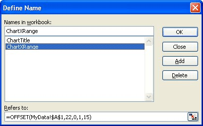
Figure 1. The New Name dialog box.

8. Enter the name Criteria, then click OK.
9. In the cell where you want a count of records meeting your criteria, enter the following:

=DCOUNT(B1:C101,2,Criteria)

Notice that the first argument used with DCOUNT is the second and third columns of your records list. This argument also includes the column labels, which are necessary so that DCOUNT can locate the proper criteria matches from the criteria table (third argument).