Please Note: This article is written for users of the following Microsoft Excel versions: 97, 2000, 2002, and 2003. If you are using a later version (Excel 2007 or later), this tip may not work for you. For a version of this tip written specifically for later versions of Excel, click here: Looking Backward through a Data Table.
Kirk has a large data table in Excel. Each row has a vehicle number, date (the table is sorted by this column), beginning mileage, and ending mileage. He would like to search backwards through the data table to find the ending mileage for the same vehicle number to use as the beginning mileage in the current row—similar to VLOOKUP but looking bottom to top rather that top to bottom.
There are several ways you can approach this with a formula. Assume, for this example, that the vehicle number is in column A, the date in column B, the starting mileage in column C, and the ending mileage in column D. What you need is a formula you can put in column C that looks up the most recent ending mileage for current vehicle. The following formula provides one approach; you should place it in cell C3:
=LOOKUP(2,1/FIND(A3,A$2:A2,1),D$2:D2)
You can copy the formula down the column as far as you need. If the vehicle number in column A has not appeared earlier in the data table, then the formula will return an error such as #VALUE! or #N/A. In that case, you can easily type over the formula with the starting mileage that you want to use for the vehicle.
Here's another formulaic approach, but this one should be entered as an array formula (by pressing Ctrl+Shift+Enter):
=IF(A3="","",MAX(IF(($A$2:A2=A3)*($D$2:D2),$D$2:D2)))
Again, place the formula in cell C3 and copy it down as far as needed. This one doesn't return an error value if the vehicle hasn't appeared earlier in the data table; it returns a value of 0. You can then type over the formula with the real starting mileage for that vehicle. The following array formula could also be used:
=IF(A3="","",INDIRECT("D"&LARGE(($A$2:A3=A3)*ROW($2:3),2)))
The difference with this array formula is that if the vehicle hasn't appeared earlier in the data table, it returns a #REF! error.
Here are two array formulas that are even shorter that you can use in C3 (and, again, copy down as needed):
=MAX((D$2:D2)*(--(A$2:A2=A3)))
=MAX(IF(A$2:A2=A3,D$2:D2))
ExcelTips is your source for cost-effective Microsoft Excel training. This tip (11744) applies to Microsoft Excel 97, 2000, 2002, and 2003. You can find a version of this tip for the ribbon interface of Excel (Excel 2007 and later) here: Looking Backward through a Data Table.

Program Successfully in Excel! This guide will provide you with all the information you need to automate any task in Excel and save time and effort. Learn how to extend Excel's functionality with VBA to create solutions not possible with the standard features. Includes latest information for Excel 2024 and Microsoft 365. Check out Mastering Excel VBA Programming today!
The VLOOKUP function is very powerful, but it will only return values that meet a very limited set of criteria. If you ...
Discover MoreThe VLOOKUP function, like other lookup functions in Excel, is not case sensitive. In other words, it doesn't matter ...
Discover MoreOne of the most useful function in Excel is VLOOKUP. One thing it won't do, however, is allow you to lookup information ...
Discover MoreFREE SERVICE: Get tips like this every week in ExcelTips, a free productivity newsletter. Enter your address and click "Subscribe."
2021-12-03 06:26:49
(see Figure 1 below)
How to use vlookup for filling the columns g,h,i for each vehicle number
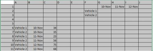
Figure 1.
2021-10-10 04:42:12
Willy Vanhaelen
Another very simple method to obtain the desired result, without formulas nor copying down, is to filter the table for the vehicle number. The last row shows the wanted mileage.
2021-10-09 10:20:39
Roy
Of course, TODAY (2021) (and in 2020, at first only if you were a beta (yeah... or alpha...) tester, er, I mean "Office Insider", of course) but after a while in 2020) the best way to do this would be to use XLOOKUP() for most searches like this. It lets you search end toward beginning so... kind of a slam dunk unless it somehow can't fit the precise situation (which does happen).
But... if you want, or need, the old school way, the LOOKUP() solution is pretty traditionally old school, but there's another old school way that works nicely and it has the advantage of its workings being more "intuitively obvious to the casual observer" (and I don't mean in the sarcastic way that was used as a joke in college around 1980) and so is easier to maintain.
It uses INDEX(). INDEX() can do many things, but one is that it can invert a range for you. The trick was slightly obtuse, but understandable, then, and even clearer now we also have SEQUENCE(). That trick is to specify the rows in reverse order.
You might think you can't, because Excel "regularizes" any range addressing you use: give it D2:A7 and it will not only make the column references A:D rather than D:A, it will also use the row references with the "proper" column order to specify the same rectangle, which looks a lot like it is switching the example's rows around as well, though you can see it isn't really. So it regularizes D2:A7 to be A2:D7. That means the usual old school trick to get a number sequence, "ROW(1:5)" to get {1,2,3,4,5} won't directly get a reverse sequence like {5,4,3,2,1} just by using "ROW(5:1)" because Excel will "fix" that to be "ROW(1:5) and give you the rising sequence instead. (That's why SEQUENCE() is so nice: it does what it's told, not what it hears. So "SEQUENCE(5,1,5,-1) gives you the falling sequence {5,4,3,2,1}, as desired.)
BUT... if you know the number of values you need (the number of "rows" you want to use in "1:x"), you can take the next higher integer and SUBTRACT the usual ("ROW(1:5)") trick. So "6-ROW(1:5)" gives you {5,4,3,2,1}. And you do usually know the number of rows just from looking at the range address you entered (or using ROWS() on the Named Range, etc.). As a minimum, you can use something complicated looking like "ROWS(A1:B5)+1-ROW(INDIRECT("1:"&ROWS(A1:B5)))" where the first two terms figure the number to subtract from and the last term builds the "ROW(1:x)" part of it.
So, say your range is E1:F5 and you'd like to search it in reverse using VLOOKUP(). For the search range parameter, use the following INDEX() function:
INDEX(E1:F5,ROWS(E1:F5)+1-ROW(INDIRECT("1:"&ROWS(E1:F5))),{1,2})
it rearranges the table from bottom to top, neatly inverting it. The last parameter in it ("{1,2}") specifies the columns and keeps them in the same order. That's what's desired in this problem. But if you want a fuller inversion, you could reverse that as well ("{2,1}"). Lots of possibilities there.
Why bother if you have XLOOKUP() handy, eh? But if you don't, or it won't fit the situation, just do the above. If you have SEQUENCE() available, use it instead of all the ROW(), ROWS(), and INDIRECT() portions.
One situation that XLOOKUP() doesn't fit so wonderfully, because it WON'T return a 2-D result (actually, to be precise, I don't think it can FORM a 2-D result, hence also cannot return one), is, well... when you need a 2-D result...
If using FILTER() to form the table that will be inverted, then unlike most times when using FILTER()'s results inside a formula, instead of basing the rows for the sequence on the rows in the range FILTER() is working upon, one needs to base it upon the number of rows FILTER() is feeding forward into the rest of the formula. Otherwise one gets extra lines of return which contain errors and that might affect one's formula's approach as it might not handle those errors in a desirable way.
Got a version of Excel that uses the menu interface (Excel 97, Excel 2000, Excel 2002, or Excel 2003)? This site is for you! If you use a later version of Excel, visit our ExcelTips site focusing on the ribbon interface.
FREE SERVICE: Get tips like this every week in ExcelTips, a free productivity newsletter. Enter your address and click "Subscribe."
Copyright © 2026 Sharon Parq Associates, Inc.
 Please Note:
This article is written for users of the following Microsoft Excel versions: 97, 2000, 2002, and 2003. If you are using a later version (Excel 2007 or later), this tip may not work for you. For a version of this tip written specifically for later versions of Excel, click here:
Please Note:
This article is written for users of the following Microsoft Excel versions: 97, 2000, 2002, and 2003. If you are using a later version (Excel 2007 or later), this tip may not work for you. For a version of this tip written specifically for later versions of Excel, click here:
Comments