Please Note: This article is written for users of the following Microsoft Excel versions: 97, 2000, 2002, and 2003. If you are using a later version (Excel 2007 or later), this tip may not work for you. For a version of this tip written specifically for later versions of Excel, click here: Averaging Values for a Given Month and Year.
George has a worksheet that includes dates (in column A) and values associated with those dates (in column B). The worksheet includes values for the last several years. He would like to calculate the average of all the values for a given month in a given year. For instance, George would like to calculate the average of all the values for May 2011.
There are several different ways to approach this problem. One way is to create a PivotTable based on your data. (PivotTables are great for aggregating and analyzing huge amounts of data.) You can easily set the value field to Average (instead of the default Sum) and group the Dates column by whatever you want.
If you'd rather not use a PivotTable, there are any number of formulas you can add to your worksheet. For instance, the following formula uses the SUMPRODUCT function to calculate the average:
=SUMPRODUCT((MONTH(A2:A1000)=5)*(YEAR(A2:A1000)=2011)*(B2:B1000)) /
(SUMPRODUCT((MONTH(A2:A1000)=5)*(YEAR(A2:A1000)=2011)*1))
The formula assumes your dates and values begin in row 2 (to allow for headings) and don't go past row 1000. If there are no dates in the data that are in the month of May 2011, then the formula returns a #DIV/0! error.
Another approach is to use an array formula, such as the following:
=AVERAGE(IF((MONTH(A2:A1000)=5)*(YEAR(A2:A1000)=2011),B2:B1000))
This approach is shorter than the SUMPRODUCT formula, but you've got to remember to hold down Ctrl+Shift+Enter as you enter the formula. You'll also get the division by zero error if there is no data for the desired month and year.
Still another approach is to use one of the database functions of Excel, DAVERAGE. All you need to do is set up a criteria table that defines what you are looking for. Assume, for example, that the headings on the columns are something original, like Date (cell A1) and Value (cell B1). You could set up a criteria table in another place, such as D1:E2. The table could look like this:
Date         Date
>4/30/11     <6/1/11
The criteria table says that you want DAVERAGE to use anything in which the Date column contains a date greater than 4/30/11 and a date less than 6/1/11. Here's the formula:
=DAVERAGE(A1:B1000,"Value",D1:E2)
The first parameter defines your database, the second parameter indicates that you want to average the information in the Value column (column B), and the third parameter tells DAVERAGE where your criteria table is located.
One quite easy way is to apply filtering of dates and use the SUBTOTAL function. Enter the following formula into a cell:
=SUBTOTAL(101,B2:B1000)
Select a cell in your data range and turn on the AutoFilter (choose Data | Filter | AutoFilter). Click the filtering arrow at the top of column A and then choose Custom Filter from the drop-down list. Excel displays the Custom AutoFilter dialog box. (See Figure 1.)
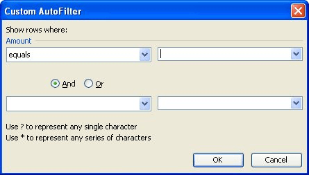
Figure 1. The Custom AutoFilter dialog box.
Use the controls in the dialog box to specify that you want records greater than 4/30/11 and less than 6/1/11. When you click on OK, only those records within May 2011 are displayed, and the subtotal formula shows the average of those visible records.
ExcelTips is your source for cost-effective Microsoft Excel training. This tip (10670) applies to Microsoft Excel 97, 2000, 2002, and 2003. You can find a version of this tip for the ribbon interface of Excel (Excel 2007 and later) here: Averaging Values for a Given Month and Year.

Solve Real Business Problems Master business modeling and analysis techniques with Excel and transform data into bottom-line results. This hands-on, scenario-focused guide shows you how to use the latest Excel tools to integrate data from multiple tables. Check out Microsoft Excel Data Analysis and Business Modeling today!
If you have a large amount of data in a worksheet and you want to extract information from the text that meets certain ...
Discover MoreIf you have a string of text that is composed of digits and non-digits, you may want to know where the digits stop and ...
Discover MorePostal codes in Canada consist of six characters, separated into two groups. This tip explains the format and then shows ...
Discover MoreFREE SERVICE: Get tips like this every week in ExcelTips, a free productivity newsletter. Enter your address and click "Subscribe."
There are currently no comments for this tip. (Be the first to leave your comment—just use the simple form above!)
Got a version of Excel that uses the menu interface (Excel 97, Excel 2000, Excel 2002, or Excel 2003)? This site is for you! If you use a later version of Excel, visit our ExcelTips site focusing on the ribbon interface.
FREE SERVICE: Get tips like this every week in ExcelTips, a free productivity newsletter. Enter your address and click "Subscribe."
Copyright © 2026 Sharon Parq Associates, Inc.
 Please Note:
This article is written for users of the following Microsoft Excel versions: 97, 2000, 2002, and 2003. If you are using a later version (Excel 2007 or later), this tip may not work for you. For a version of this tip written specifically for later versions of Excel, click here:
Please Note:
This article is written for users of the following Microsoft Excel versions: 97, 2000, 2002, and 2003. If you are using a later version (Excel 2007 or later), this tip may not work for you. For a version of this tip written specifically for later versions of Excel, click here:
Comments