Alerts About Approaching Due Dates

Jonathan developed a worksheet that tracks due dates for various departmental documents. He wondered if there was a way for Excel to somehow alert him if the due date for a particular document was approaching.

There are several ways that this can be done in Excel, and you should pick the method that is best for your purposes. The first method is to simply add a column to your worksheet that will be used for the alert. Assuming your due date is in column F, you could place the following type of formula in column G:

=IF(F3<(TODAY()+7),"<<<","")

The formula checks to see if the date in cell F3 is earlier than a week from today. If so, then the formula displays "<<<" in the cell. The effect of this formula is to alert you to any date that is either past or within the next week.

Another approach is to use the conditional formatting capabilities of Excel. Follow these steps:

1. Select the cells that contain the document due dates.
2. Choose Conditional Formatting from the Format menu. Excel displays the Conditional Formatting dialog box.
3. Make sure the first drop-down list is "Cell Value Is." (This should be the default.) (See Figure 1.)



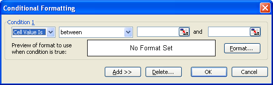
Figure 1. The Conditional Formatting dialog box.

4. Make sure the second drop-down list is "Less Than."
5. In the formula area, enter "=TODAY()" (without the quote marks).
6. Click the Format button. Excel displays the Format Cells dialog box. (See Figure 2.)



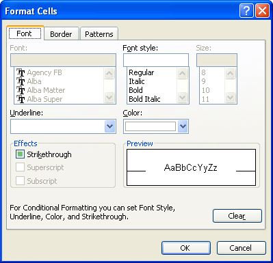
Figure 2. The Format Cells dialog box.

7. Using the Color drop-down list, choose the color red.
8. Click OK to close the Format Cells dialog box.
9. Click Add. The Conditional Format dialog box expands to include a second condition.
10. Make sure the first drop-down list for the second condition is "Cell Value Is." (This should be the default.)
11. Make sure the second drop-down list is "Less Than."
12. In the formula area, enter "=TODAY()+7" (without the quote marks).
13. Click the Format button. Excel displays the Format Cells dialog box.
14. Using the Color drop-down list, choose the color blue.
15. Click OK to close the Format Cells dialog box. (See Figure 3.)



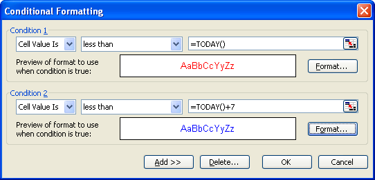
Figure 3. The finished Conditional Formatting dialog box.

16. Click OK to close the Conditional Formatting dialog box.

This is a two-tiered format, and you end up with two levels of alert. If the due date is already past, then it shows up as red. If the due date is today or within the next seven days, then it shows up in blue.

ExcelTips is your source for cost-effective Microsoft Excel training. This tip (3179) applies to Microsoft Excel 97, 2000, 2002, and 2003. You can find a version of this tip for the ribbon interface of Excel (Excel 2007 and later) here: Alerts About Approaching Due Dates.