Please Note: This article is written for users of the following Microsoft Excel versions: 97, 2000, 2002, and 2003. If you are using a later version (Excel 2007 or later), this tip may not work for you. For a version of this tip written specifically for later versions of Excel, click here: Non-adjusting References in Formulas.
Everybody knows you can enter a formula in Excel. (What would a spreadsheet be without formulas, after all?) If you use address references in a formula, those references are automatically updated if you insert or delete cells, rows, or columns and those changes affect the address reference in some way. Consider, for example, the following simple formula:
=IF(A7=B7,"YES","NO")
If you insert a cell above B7, then the formula is automatically adjusted by Excel so that it appears like this:
=IF(A7=B8,"YES","NO")
What if you don?t want Excel to adjust the formula, however? You might try adding some dollar signs to the address, but this only affects addresses in formulas that are later copied; it doesn?t affect the formula itself if you insert or delete cells that affect the formula.
The best way to make the formula references ?non-adjusting? is to modify the formula itself to use different worksheet functions. For instance, you could use this formula in cell C7:
=IF(INDIRECT("A"&ROW(C7))=INDIRECT("B"&ROW(C7)),"YES","NO")
What this formula does is to construct an address based on whatever cell the formula appears in. The ROW function returns the row number of the cell (C7 in this case, so the value 7 is returned) and then the INDIRECT function is used to reference the constructed address, such as A7 and B7. If you insert (or delete) cells above A7 or B7, the reference in cell C7 is not disturbed, as it just blithely constructs a brand new address.
Another approach is to use the OFFSET function to construct a similar type of reference:
=IF(OFFSET($A$1,ROW()-1,0)=OFFSET($B$1,ROW()-1,0),"YES","NO")
This formula simply looks at where it is (in column C) and compares the values in the cells that are to its left. This formula is similarly undisturbed if you happen to insert or delete cells in either column A or B.
A final approach (and perhaps the slickest one) is to use named formulas. This is a feature of Excel?s naming capabilities that is rarely used by most people. Follow these steps:
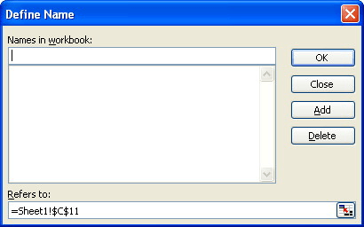
Figure 1. The Define Name dialog box.
=IF(A2=B2,"YES","NO")
At this point you?ve created your named formula. You can now use it in any cell in column C in this manner:
=CompareMe
It compares whatever is in the two cells to its left, just as your original formula was designed to do. Better still, the formula is not automatically adjusted as you insert or delete cells.
�����������������������������������������������������������������������������������������������������������������������������������������������������������������������������������������������������������������������������������������������������������������������������������������������������������������������������������������������������������������������������������������������������������������������������������������������������������������������������������������������������������������������������������������������������������������������������������������������������������������������������������������������������������������������������������������������������������������������������������������������������������������������������������������������������������������������������������������������������������������������������������������������������������������������������������������������������������������������������������������������������������������������������������������������������������������������������������������������������������������������������������������������������������������������������������������������������������������������������������������������������������������������������������������������������������������������������������������������������������������������������������������������������������������������������������������������������������������������������������������������������������������������������������������������������������������������������������������������������������������������������������������������������������������������������������������������������������������������������������������������������������������������������������������������������������������������������������������������������������������������������������������������������������������������������������������������������������������������������������������������������������������������������������������������������������������������������������������������������������������������������������������������������������������������������������������������������������������������������������������������������������������������������������������������������������������������������������������������������������������������������������������������������������������������������������������������������������������������������������������������������������������������������������������������������������������������������������������������������������������������������������������������������������������������������������������������������������������������������������������������������������������������������������������������������������������������������������������������������������������������������������������������������������������������������������������������������������������������������������������������������������������������������������������������ExcelTips is your source for cost-effective Microsoft Excel training. This tip (2876) applies to Microsoft Excel 97, 2000, 2002, and 2003. You can find a version of this tip for the ribbon interface of Excel (Excel 2007 and later) here: Non-adjusting References in Formulas.

Program Successfully in Excel! This guide will provide you with all the information you need to automate any task in Excel and save time and effort. Learn how to extend Excel's functionality with VBA to create solutions not possible with the standard features. Includes latest information for Excel 2024 and Microsoft 365. Check out Mastering Excel VBA Programming today!
In mathematics, the sum of a range of sequential integers, starting with 1, is known as a triangular number or Gaussian ...
Discover MoreYou can use some of Excel's worksheet functions across a range or worksheets, but not all of them. One that has problems ...
Discover MoreFiguring out how to average data that is in a contiguous range of cells is easy. When the data is spread over a group of ...
Discover MoreFREE SERVICE: Get tips like this every week in ExcelTips, a free productivity newsletter. Enter your address and click "Subscribe."
2020-10-31 15:45:54
I really like your defined named Solution but I don't think it works in my situation wondering if you could possibly give me a tip ???
I have a fairly large balance type sheet where I am taking some monthly totals in columns M,N,O,P, and Q. Let's focus on Column Q. There is a column L where I have the formula =J-Q. So at the end of the month I insert 5 new blank columns and move colum Q over to column V. So Column L now has the formula =J-V. I need column L to have the formula =J-V-Q. I hope that explains it.
Got a version of Excel that uses the menu interface (Excel 97, Excel 2000, Excel 2002, or Excel 2003)? This site is for you! If you use a later version of Excel, visit our ExcelTips site focusing on the ribbon interface.
FREE SERVICE: Get tips like this every week in ExcelTips, a free productivity newsletter. Enter your address and click "Subscribe."
Copyright © 2026 Sharon Parq Associates, Inc.
 Please Note:
This article is written for users of the following Microsoft Excel versions: 97, 2000, 2002, and 2003. If you are using a later version (Excel 2007 or later), this tip may not work for you. For a version of this tip written specifically for later versions of Excel, click here:
Please Note:
This article is written for users of the following Microsoft Excel versions: 97, 2000, 2002, and 2003. If you are using a later version (Excel 2007 or later), this tip may not work for you. For a version of this tip written specifically for later versions of Excel, click here:
Comments