Understanding Views

A view is a pattern for what information within a worksheet should look like. This pattern can be given a name and saved within Excel. The named view can later be recalled quickly. In some ways a view is similar to a scenario. (Scenarios are discussed in other issues of ExcelTips.) They differ, however, in that a scenario deals with the content (the values) stored in a worksheet, while a view is concerned with how the worksheet appears.

A view can contain information such as which rows and columns are visible, row height, column width, formatting characteristics, and window size and position. You can define and store several views of data in a worksheet. For instance, one view could show the entire worksheet, while another could show a condensed (or summary) view of the information. Still another could be used to show the full worksheet on the screen at one time.

To create a view, follow these steps:

1. Format and situate your worksheet as you want it to appear.
2. Choose Custom Views from the View menu. Excel displays the Custom Views dialog box.
3. Click on the Add button. Excel displays the Add View dialog box. (See Figure 1.)



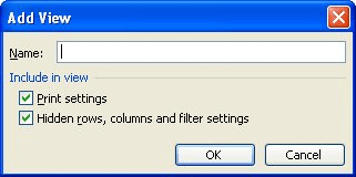
Figure 1. The Add View dialog box.

4. In the Name field, supply the name you want associated with this view. This name can be up to 255 characters long, including spaces.
5. In the View Includes section, select the options that reflect what you want saved with this view. You can choose to include both print settings and hidden rows and columns.
6. When you are satisfied with your settings, click the OK button. The current view is saved by Excel.

You can now proceed to adjust the formatting and display of your worksheet, so it reflects what you want saved as the next view. Repeat this process to store the new view.

ExcelTips is your source for cost-effective Microsoft Excel training. This tip (2865) applies to Microsoft Excel 97, 2000, 2002, and 2003. You can find a version of this tip for the ribbon interface of Excel (Excel 2007 and later) here: Understanding Views.