Please Note: This article is written for users of the following Microsoft Excel versions: 97, 2000, 2002, and 2003. If you are using a later version (Excel 2007 or later), this tip may not work for you. For a version of this tip written specifically for later versions of Excel, click here: Selecting Random Names.
A common task for many people is to pick a number of random names from a large list. For instance, you may be running a contest for your community, and you have 1,000 people that have entered. With their names in each row of a table, you may be wondering how to select a certain number of the names randomly.
As is often the case with Excel, there are a number of different approaches you can take. Each approach examined in this tip assumes that the names you need to select from are listed in cells A1 through A1000. Of course, your range of names could be shorter or longer, but the point is that they are in contiguous cells in column A. The examples also assume that you need to select 15 names at random from the list.
The first approach is to use the INDEX function. Enter the following formula in cells B1:B15:
=INDEX(A:A,INT((RAND()*1000)+1),1)
A similar formula uses the OFFSET function:
=OFFSET($A$1,ROUNDUP(RAND()*1000,0),0,1,1)
It is possible, but not probable, that you will get the same name twice in the resulting list. (The improbability comes because of the size of the original list. The larger the list, the less probable there will be duplicates in the extracted list.) If you do get a duplicate name, then simply force a recalculation of your worksheet by pressing F9. Each time your recalculate, the list of extracted names is regenerated.
Another potential approach requires the use of multiple columns. Simply follow these steps:
=RANK(B1,$B$1:$B$1000)
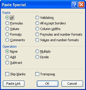
Figure 1. The Paste Special dialog box.
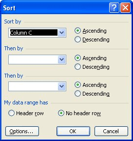
Figure 2. The Sort dialog box.
The result is that column C now contains a ranking of all the random numbers in column B. The first 15 rows contain your random names.
In this approach you could also have left out column C completely and simply sorted your list based on the static random values in column B. Again, the top 15 would be your random names.
Of course, there are any number of macro solutions you could use for this problem. The coding of any macro will be similar, relying on VBA's RND function to generate random numbers. Of all the possible macro solutions, perhaps the following is the most unique and offers some advantages not available with the workbook solutions discussed so far:
Sub GetRandom()
    Dim iRows As Integer
    Dim iCols As Integer
    Dim iBegRow As Integer
    Dim iBegCol As Integer
    Dim J As Integer
    Dim sCells As String

    Set TempDO = New DataObject

    iRows = Selection.Rows.Count
    iCols = Selection.Columns.Count
    iBegRow = Selection.Row
    iBegCol = Selection.Column

    If iRows < 16 Or iCols > 1 Then
        MsgBox "Too few rows or too many columns"
    Else
        Randomize Timer
        sCells = ""
        For J = 1 To 15
            iWantRow = Int(Rnd() * iRows) + iBegRow
            sCells = sCells & Cells(iWantRow, iBegCol) & vbCrLf
        Next J
        TempDO.SetText sCells
        TempDO.PutInClipboard
    End If
End Sub
To use this macro, just select the names from which you want to select the 15 random names. In the examples thus far, you would select the range A1:A1000. The macro then pulls 15 names at random from the cells, and puts them in the Clipboard. When you run the macro, you can then paste the contents of the Clipboard where ever you want. Every time the macro is run, a different group of 15 is selected.
Note:
ExcelTips is your source for cost-effective Microsoft Excel training. This tip (2811) applies to Microsoft Excel 97, 2000, 2002, and 2003. You can find a version of this tip for the ribbon interface of Excel (Excel 2007 and later) here: Selecting Random Names.

Create Custom Apps with VBA! Discover how to extend the capabilities of Office 365 applications with VBA programming. Written in clear terms and understandable language, the book includes systematic tutorials and contains both intermediate and advanced content for experienced VB developers. Designed to be comprehensive, the book addresses not just one Office application, but the entire Office suite. Check out Mastering VBA for Microsoft Office 365 today!
Different professions use numbers in entirely unique ways. You may need to come up with a number that represents the ...
Discover MoreWhen working with dates and the relationship between dates, Excel provides a variety of worksheet functions that may ...
Discover MoreWhen you filter data, Excel displays only a portion of what is really in a worksheet. If you want to count the number of ...
Discover MoreFREE SERVICE: Get tips like this every week in ExcelTips, a free productivity newsletter. Enter your address and click "Subscribe."
There are currently no comments for this tip. (Be the first to leave your comment—just use the simple form above!)
Got a version of Excel that uses the menu interface (Excel 97, Excel 2000, Excel 2002, or Excel 2003)? This site is for you! If you use a later version of Excel, visit our ExcelTips site focusing on the ribbon interface.
FREE SERVICE: Get tips like this every week in ExcelTips, a free productivity newsletter. Enter your address and click "Subscribe."
Copyright © 2026 Sharon Parq Associates, Inc.
 Please Note:
This article is written for users of the following Microsoft Excel versions: 97, 2000, 2002, and 2003. If you are using a later version (Excel 2007 or later), this tip may not work for you. For a version of this tip written specifically for later versions of Excel, click here:
Please Note:
This article is written for users of the following Microsoft Excel versions: 97, 2000, 2002, and 2003. If you are using a later version (Excel 2007 or later), this tip may not work for you. For a version of this tip written specifically for later versions of Excel, click here:
Comments