Please Note: This article is written for users of the following Microsoft Excel versions: 97, 2000, 2002, and 2003. If you are using a later version (Excel 2007 or later), this tip may not work for you. For a version of this tip written specifically for later versions of Excel, click here: Sorting Dates by Month.
There may come a time when you have a need to sort a list of information based on the month represented in a particular column. For instance, you may have a list of people and their birthdays, and you want to sort the list by birthday month so that you know whose birthdays occur within a particular month.
The easiest way to do this is to add a new column to your table. This column will be named something descriptive, such as "Birth Month" or simply "Month." For instance, let's say that you have people's birthdays in column B, you could add the new column in column C. In this column you could then use the MONTH function, as follows:
=MONTH(B3)
This particular formula would go in cell C3, but similar formulas would go in each cell of column C. The result is that column C will contain numbers ranging between 1 and 12, representing to birth months of the people. You can now sort the list based on the contents of column C, with the result that the list is sorted by month.
This approach works fine, but you may not be able to add another column to your worksheet. If this is the case, you can follow these steps to sort by month:
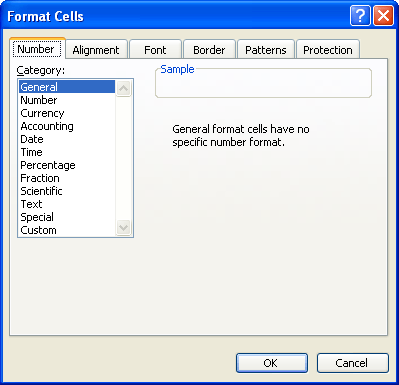
Figure 1. The Number tab of the Format Cells dialog box.
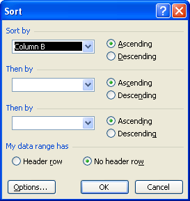
Figure 2. The Sort dialog box.
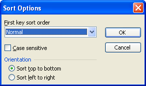
Figure 3. The Sort Options dialog box.
You may be wondering why you need to reformat the display of the cells containing the birthdates (steps 1 through 6). The reason is that when you finally sort your list (steps 7 through 13), if you simply have the original full dates displayed, Excel will effectively sort the list chronologically rather than by month.
There is an additional way you can approach the problem. This involves actually converting the dates into text (instead of the internal serial numbers), as follows:
Your dates are now pasted into Excel as true text entries, not as dates. This allows you to easily sort the information according to the month in the date.
ExcelTips is your source for cost-effective Microsoft Excel training. This tip (3183) applies to Microsoft Excel 97, 2000, 2002, and 2003. You can find a version of this tip for the ribbon interface of Excel (Excel 2007 and later) here: Sorting Dates by Month.

Professional Development Guidance! Four world-class developers offer start-to-finish guidance for building powerful, robust, and secure applications with Excel. The authors show how to consistently make the right design decisions and make the most of Excel's powerful features. Check out Professional Excel Development today!
If you need to know how a range of data is sorted, the task is not as easy as you might at first think. This tip examines ...
Discover MoreGot a huge amount of data you need to sort in a worksheet, but Excel doesn't seem to be sorting it correctly? Here's some ...
Discover MoreWant to sort addresses by even and odd numbers? By using a formula and doing a little sorting, Excel can return the ...
Discover MoreFREE SERVICE: Get tips like this every week in ExcelTips, a free productivity newsletter. Enter your address and click "Subscribe."
There are currently no comments for this tip. (Be the first to leave your comment—just use the simple form above!)
Got a version of Excel that uses the menu interface (Excel 97, Excel 2000, Excel 2002, or Excel 2003)? This site is for you! If you use a later version of Excel, visit our ExcelTips site focusing on the ribbon interface.
FREE SERVICE: Get tips like this every week in ExcelTips, a free productivity newsletter. Enter your address and click "Subscribe."
Copyright © 2026 Sharon Parq Associates, Inc.
 Please Note:
This article is written for users of the following Microsoft Excel versions: 97, 2000, 2002, and 2003. If you are using a later version (Excel 2007 or later), this tip may not work for you. For a version of this tip written specifically for later versions of Excel, click here:
Please Note:
This article is written for users of the following Microsoft Excel versions: 97, 2000, 2002, and 2003. If you are using a later version (Excel 2007 or later), this tip may not work for you. For a version of this tip written specifically for later versions of Excel, click here:
Comments