Please Note: This article is written for users of the following Microsoft Excel versions: 97, 2000, 2002, and 2003. If you are using a later version (Excel 2007 or later), this tip may not work for you. For a version of this tip written specifically for later versions of Excel, click here: Creating 3-D Formatting for a Cell.
Written by Allen Wyatt (last updated April 20, 2024)
This tip applies to Excel 97, 2000, 2002, and 2003
Do you want the formatting of a cell to "stand out" from the surrounding cells? It's rather easy to do, once you understand how to create the illusion of three dimensions. Follow these steps:
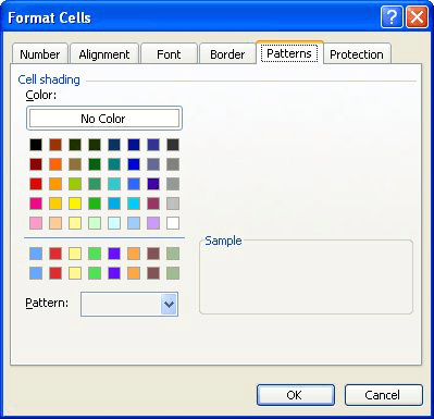
Figure 1. The Patterns tab of the Format Cells dialog box.
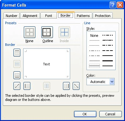
Figure 2. The Border tab of the Format Cells dialog box.
The cell you selected in step 1 should now look as if it is "raised" off the worksheet around it. You can accentuate the effect even more if you apply a background color to the cells that surround the one that you want to look raised.
ExcelTips is your source for cost-effective Microsoft Excel training. This tip (3061) applies to Microsoft Excel 97, 2000, 2002, and 2003. You can find a version of this tip for the ribbon interface of Excel (Excel 2007 and later) here: Creating 3-D Formatting for a Cell.

Excel Smarts for Beginners! Featuring the friendly and trusted For Dummies style, this popular guide shows beginners how to get up and running with Excel while also helping more experienced users get comfortable with the newest features. Check out Excel 2013 For Dummies today!
You can shade your cells by filling them with a pattern. Here's how to select the pattern you want used.
Discover MoreIf your column headings are too large to work well in your worksheet, why not turn them a bit? Here's how.
Discover MoreExcel's conditional formatting feature allows you to create formats that are based on a wide variety of criteria. If you ...
Discover MoreFREE SERVICE: Get tips like this every week in ExcelTips, a free productivity newsletter. Enter your address and click "Subscribe."
There are currently no comments for this tip. (Be the first to leave your comment—just use the simple form above!)
Got a version of Excel that uses the menu interface (Excel 97, Excel 2000, Excel 2002, or Excel 2003)? This site is for you! If you use a later version of Excel, visit our ExcelTips site focusing on the ribbon interface.
FREE SERVICE: Get tips like this every week in ExcelTips, a free productivity newsletter. Enter your address and click "Subscribe."
Copyright © 2024 Sharon Parq Associates, Inc.
 Please Note:
This article is written for users of the following Microsoft Excel versions: 97, 2000, 2002, and 2003. If you are using a later version (Excel 2007 or later), this tip may not work for you. For a version of this tip written specifically for later versions of Excel, click here:
Please Note:
This article is written for users of the following Microsoft Excel versions: 97, 2000, 2002, and 2003. If you are using a later version (Excel 2007 or later), this tip may not work for you. For a version of this tip written specifically for later versions of Excel, click here:
Comments