Pulling All Fridays

When developing a worksheet to track business information, you may have a need to determine all the Fridays in a range of dates. The best way to do this depends on the data in your worksheet and the way in which you want results displayed.

If you have a list of dates in a column, you can use several different worksheet functions to determine whether those dates are Fridays or not. The WEEKDAY function returns a number, 1 through 7, depending on the weekday of the date used as an argument:

=WEEKDAY(A2)

This usage returns the number 6 if the date in A2 is a Friday. If this formula is copied down next to a column of dates, you could then use the AutoFilter feature of Excel to show only those dates where the weekday is 6 (Friday).

You could also use the conditional formatting feature of Excel to simply highlight all the Fridays in a list of dates. Follow these steps:

1. Select the list of dates.
2. Choose Conditional Formatting from the Format menu. Excel displays the Conditional Formatting dialog box.
3. Use the Condition drop-down to choose Formula Is. (See Figure 1.)



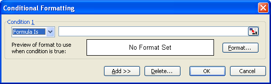
Figure 1. The Conditional Formatting dialog box.

4. In the formula area, to the right of the drop-down list used in step 3, enter the following formula, replacing A2 with the address of the active cell selected in step 1:

     =WEEKDAY(A2)=6

5. Click Format to display the Format Cells dialog box.
6. Set the formatting options to highlight the Fridays as desired.
7. Click OK to dismiss the Format Cells dialog box. The formatting you specified in step 6 should now appear in the preview area for the condition.
8. Click OK.

If you want to determine a series of Fridays based on a beginning and ending date, you can set up a series of formulas to figure them out. Assuming that the beginning date is in A2 and the ending date is in A3, you can use the following formula to figure out the date of the first Friday:

=IF(A2+IF(WEEKDAY(A2)<=6,6-WEEKDAY(A2),6)>A3,
"",A2+IF(WEEKDAY(A2)<=6,6-WEEKDAY(A2),6))

If you place this formula in cell C2 and then format it as a date, you can use the following formula to determine the next Friday in the range:

=IF(C2="","",IF(C2+7>$A$3,"",C2+7))

If you copy this formula down for a bunch of cells, you end up with a list of Fridays between whatever range of dates is specified by A2 and A3.

If you actually want to "pull" Fridays in a specific date range, then you will need to use a macro. There are several ways you can go about this. This simple macro will examine all the dates in the range A2:A24. If they are Fridays, then the date is copied into column C, beginning at C2. The result, of course, is that the list starting at C2 will only contain dates that are Fridays.

Sub PullFridays1()
    Dim dat As Range
    Dim c As Range
    Dim rw As Integer

    Set dat = ActiveSheet.Range("A2:A24")
    rw = 2
    For Each c In dat
        If Weekday(c) = vbFriday Then
            Cells(rw, 3).Value = Format(c)
            rw = rw + 1
        End If
    Next
End Sub

If desired, you can change the range examined by the macro simply by changing the A2:A24 reference, and you can change where the dates are written by changing the value of rw (the row) and the value 3 (the column) in the Cells function.

If you would rather work with a beginning date and an ending date, you can modify the macro so that it will step through the dates. The following macro assumes that the beginning date is in cell A2 and the ending date is in cell A3.

Sub PullFridays2()
    Dim dStart As Date
    Dim dEnd As Date
    Dim rw As Integer

    dStart = Range("A2").Value
    dEnd = Range("A3").Value

    rw = 2
    While dStart < dEnd
        If Weekday(dStart) = vbFriday Then
            Cells(rw, 3).Value = dStart
            Cells(rw, 3).NumberFormat = "m/d/yyyy"
            rw = rw + 1
        End If
        dStart = dStart + 1
    Wend
End Sub

The macro still pulls the Fridays from the range and places them into a list starting at C2.

Another macro approach is to create a user-defined function that returns specific Fridays within a range. The following does just that:

Function PullFridays3(dStartDate As Date, _
                      dEndDate As Date, _
                      iIndex As Integer)
    Dim iMaxDays As Integer
    Dim dFirstday As Date

    Application.Volatile
    If dStartDate > dEndDate Then
        PullFridays3 = CVErr(xlErrNum)
        Exit Function
    End If

    dFirstday = vbFriday - Weekday(dStartDate) + dStartDate
    If dFirstday < dStartDate Then dFirstday = dFirstday + 7
    iMaxDays = Int((dEndDate - dFirstday) / 7) + 1

    PullFridays3 = ""
    If iIndex = 0 Then
        PullFridays3 = iMaxDays
    ElseIf iIndex <= iMaxDays Then
        PullFridays3 = dFirstday + (iIndex - 1) * 7
    End If
End Function

You use this function in a cell in your worksheet in the following manner:

=PULLFRIDAYS3(A2,A3,1)

The first argument for the function is the starting date and the second is the ending date. The third argument indicates which Friday you want returned from within the specified range. If you use 1, you get the first Friday, 2 returns the second Friday, etc. If you use a 0 for the third argument, then the function returns the number of Fridays in the specified range. If the specified beginning date is greater than the ending date, then the function returns a #NUM error.

ExcelTips is your source for cost-effective Microsoft Excel training. This tip (2930) applies to Microsoft Excel 97, 2000, 2002, and 2003. You can find a version of this tip for the ribbon interface of Excel (Excel 2007 and later) here: Pulling All Fridays.