Unique Date Displays

Jon requested help on how to subtract two dates and display the result such that the years were on the left of the decimal and the months on the right. Thus, if you subtracted January 7, 1985 from August 12, 2009, the result would be 24.7.

The easiest way to do this is to simply do your date subtractions as regular, and then use a custom format to display the result. For instance, if the lower date were in cell A2 and the higher date in B2, you could use the following formula in C2:

=B2-A2

You would then follow these steps to format the display of the result in cell C2:

1. Select the cell. (In this case, cell C2.)
2. Choose Cells from the Format menu. Excel displays the Format Cells dialog box.
3. Make sure the Number tab is selected.
4. In the Category list, at the left side of the dialog box, choose Custom. (See Figure 1.)



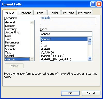
Figure 1. The Number tab of the Format Cells dialog box.

5. In the Type box, at the left of the dialog box, enter the following format: yy.m
6. Click on OK.

The result is that C2 shows the number of years to the left of the decimal and the number of months to the right. The problem with this is that it will always vary the number of months from 1 to 12, rather than 0 to 11, as one would expect if you were looking for elapsed months.

To overcome this, you could enter the following formula in cell C2:

=(YEAR(B2)-YEAR(A2))+(MONTH(B2)-MONTH(A2))/100

This formula returns the number of years on the left of the decimal and the number of months on the right. The months are always expressed using two decimal places, however. If you wanted to make sure that the months were expressed with no leading zeros, then you would use this formula variation:

=VALUE(ABS(YEAR(B2)-YEAR(A2)) & "." & ABS(MONTH(B2)-MONTH(A2)))

ExcelTips is your source for cost-effective Microsoft Excel training. This tip (2182) applies to Microsoft Excel 97, 2000, 2002, and 2003. You can find a version of this tip for the ribbon interface of Excel (Excel 2007 and later) here: Unique Date Displays.