Using a Numeric Portion of a Cell in a Formula

Rita described a problem where she is provided information, in an Excel worksheet, that combines both numbers and alphabetic characters in a cell. In particular, a cell may contain "3.5 V", which means that 3.5 hours of vacation time was taken. (The character at the end of the cell could change, depending on the type of hours the entry represented.) Rita wondered if it was possible to still use the data in a formula in some way.

Yes, it is possible, and there are several ways to approach the issue. The easiest way (and cleanest) would be to simply move the alphabetic characters to their own column. Assuming that the entries will always consist of a number, followed by a space, followed by the characters, you can do the "splitting" this way:

1. Make sure there is a blank column to the right of the entries.
2. Select the entries.
3. Choose Text to Columns from the Data menu. Excel displays the first step of the Convert Text to Columns Wizard. (See Figure 1.)



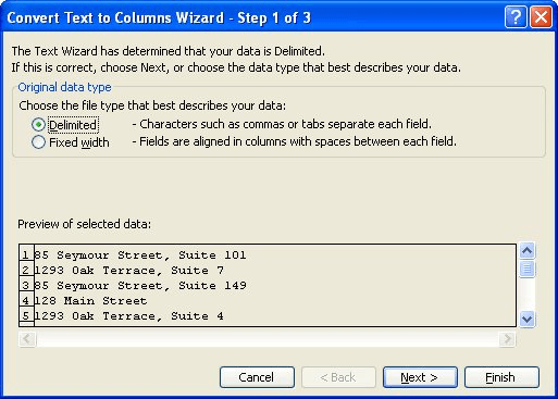
Figure 1. The first step of the Convert Text to Columns Wizard.

4. The Delimited radio button should be selected. Click Next. Excel displays the second step of the wizard.
5. Make sure the Space check box is selected, then click Next. Excel displays the third step of the wizard.
6. Click Finish.

Word splits the entries into two columns, with the numbers in the leftmost column and the alphabetic characters in the right. You can then any regular math functions on the numeric values that you desire.

If it is not feasible to separate the data into columns (perhaps your company doesn't allow such a division, or it may cause problems with those later using the worksheet), then you can approach the problem in a couple of other ways.

First, you could use the following formula on individual cells:

=VALUE(LEFT(A3,LEN(A3)-2))

The LEFT function is used to strip off the two rightmost characters (the space and the letter) of whatever is in cell A3, and then the VALUE function converts the result to a number. You can then use this result as you would any other numeric value.

If you want to simply sum the column containing your entries, you could use an array formula. Enter the following in a cell:

=SUM(VALUE(LEFT(A3:A21,LEN(A3:A21)-2)))

Make sure you actually enter the formula by pressing Shift+Ctrl+Enter. Because this is an array formula, the LEFT and VALUE functions are applied to each cell in the range A3:A21 individually, and then summed using the SUM function.

ExcelTips is your source for cost-effective Microsoft Excel training. This tip (3185) applies to Microsoft Excel 97, 2000, 2002, and 2003. You can find a version of this tip for the ribbon interface of Excel (Excel 2007 and later) here: Using a Numeric Portion of a Cell in a Formula.