Written by Allen Wyatt (last updated August 11, 2018)
This tip applies to Excel 97, 2000, 2002, and 2003
Excel includes a powerful feature that allow you to format the contents of a cell based on a set of conditions that you specify. This is know as conditional formatting. The first step in using conditional formatting, of course, is to select the cell whose formatting should be conditional. Then choose Conditional Formatting from the Format menu. Excel displays the Conditional Formatting dialog box. (See Figure 1.)
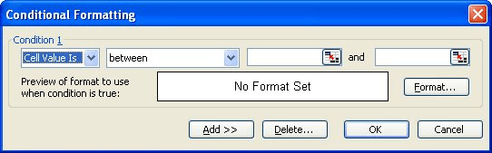
Figure 1. The Conditional Formatting dialog box.
The top line of the dialog box is where you specify the condition for which you want Excel to test. There are two types of conditions you can test, and they are specified in the first pull-down list of the dialog box. You can have Excel test the cell value (Cell Value Is), or evaluate a formula (Formula Is). Each of these are quite different in their effect.
When the first pull-down list of a condition is set to Cell Value Is, you can specify thresholds for the result shown in the cell. You then use the second pull-down list to specify how Excel should examine the cell value. You can choose from any of the following:
These test conditions cover the entire gamut of how your cell could be viewed. When you specify a test, you can then specify the actual values to test for. For instance, if you wanted Excel to apply a particular format if the value in the cell exceeds 500, then you would choose Greater Than as your test, and enter 500 in the field just to the right of the test.
When the first pull-down list of a condition is set to Formula Is, you can specify a particular formula for determining if special formatting should be applied to the cell. This is most useful if the formatting is based on a value in a cell different from the one you selected when you first chose Conditional Formatting from the Format menu.
For instance, let's say that column A has a list of company names, and column N has a total of all the purchases made by that company during the year. You may want the company name to appear in bold, red type if their sales exceeded a certain amount. This type of scenario is perfect for using a formula for your conditional test. The reason is because the formatting in column A will be based not on column A, but on a value in column N.
To complete your conditional test, select Formula Is in the pull-down list, and then enter your formula in the space provided in the dialog box. Formulas must evaluate to either a true or false condition, not to some other value. For instance, you could use the formula =N4>500 if you wanted cell A4 to be conditionally formatted if cell N4 exceeds a value of 500.
ExcelTips is your source for cost-effective Microsoft Excel training. This tip (2795) applies to Microsoft Excel 97, 2000, 2002, and 2003.
Excel Smarts for Beginners! Featuring the friendly and trusted For Dummies style, this popular guide shows beginners how to get up and running with Excel while also helping more experienced users get comfortable with the newest features. Check out Excel 2013 For Dummies today!
Conditional formatting is a great feature in Excel. Unfortunately, you can't sort or filter by the results of that ...
Discover MoreConditional formatting can be used to draw attention to all sorts of data based upon the criteria you specify. Here's how ...
Discover MoreConditional formatting is very powerful, but at some point you may want to make the formatting "unconditional." In other ...
Discover MoreFREE SERVICE: Get tips like this every week in ExcelTips, a free productivity newsletter. Enter your address and click "Subscribe."
There are currently no comments for this tip. (Be the first to leave your comment—just use the simple form above!)
Got a version of Excel that uses the menu interface (Excel 97, Excel 2000, Excel 2002, or Excel 2003)? This site is for you! If you use a later version of Excel, visit our ExcelTips site focusing on the ribbon interface.
FREE SERVICE: Get tips like this every week in ExcelTips, a free productivity newsletter. Enter your address and click "Subscribe."
Copyright © 2024 Sharon Parq Associates, Inc.
Comments