Please Note: This article is written for users of the following Microsoft Excel versions: 97, 2000, 2002, and 2003. If you are using a later version (Excel 2007 or later), this tip may not work for you. For a version of this tip written specifically for later versions of Excel, click here: Conditional Formatting Based on Date Proximity.
Richard wondered if it was possible, using conditional formatting, to change the color of a cell. For his purposes he wanted a cell to be red if it contains today's date, to be yellow if it contains a date within a week of today, and to be green if it contains a date within two weeks.
You can achieve this type of conditional formatting if you apply a formula. For instance, let's assume that you want to apply the conditional formatting to cell A1. Just follow these steps:
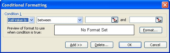
Figure 1. The Conditional Formatting dialog box.

Figure 2. The Patterns tab of the Format Cells dialog box.
One important thing to bear in mind with conditional formatting is that criteria are evaluated in the order in which they appear. Once a criteria has been met, then the formatting is applied and other criteria are not tested. It is therefore important to set out the tests in the correct order. If, in the example above, the criteria had been entered in the reverse order, i.e. test for 14 days, then 7 and then 0, it would have only applied the 14 days format even if the date entered was today. In other words, if the date is today then all three of the tests would have been met so you have to be careful of the order in order to get the result you need.
ExcelTips is your source for cost-effective Microsoft Excel training. This tip (2664) applies to Microsoft Excel 97, 2000, 2002, and 2003. You can find a version of this tip for the ribbon interface of Excel (Excel 2007 and later) here: Conditional Formatting Based on Date Proximity.

Dive Deep into Macros! Make Excel do things you thought were impossible, discover techniques you won't find anywhere else, and create powerful automated reports. Bill Jelen and Tracy Syrstad help you instantly visualize information to make it actionable. You�ll find step-by-step instructions, real-world case studies, and 50 workbooks packed with examples and solutions. Check out Microsoft Excel 2019 VBA and Macros today!
Conditional formatting is a great tool. You may need to use this tool to tell the difference between cells that are empty ...
Discover MoreTired of the default colors that Excel uses to display the row and column coordinates? You can modify the colors, but ...
Discover MoreConditional formatting is a great feature in Excel. Here's how you can copy conditional formats from one cell to another ...
Discover MoreFREE SERVICE: Get tips like this every week in ExcelTips, a free productivity newsletter. Enter your address and click "Subscribe."
There are currently no comments for this tip. (Be the first to leave your comment—just use the simple form above!)
Got a version of Excel that uses the menu interface (Excel 97, Excel 2000, Excel 2002, or Excel 2003)? This site is for you! If you use a later version of Excel, visit our ExcelTips site focusing on the ribbon interface.
FREE SERVICE: Get tips like this every week in ExcelTips, a free productivity newsletter. Enter your address and click "Subscribe."
Copyright © 2026 Sharon Parq Associates, Inc.
 Please Note:
This article is written for users of the following Microsoft Excel versions: 97, 2000, 2002, and 2003. If you are using a later version (Excel 2007 or later), this tip may not work for you. For a version of this tip written specifically for later versions of Excel, click here:
Please Note:
This article is written for users of the following Microsoft Excel versions: 97, 2000, 2002, and 2003. If you are using a later version (Excel 2007 or later), this tip may not work for you. For a version of this tip written specifically for later versions of Excel, click here:
Comments